-
【3D图像分割】基于 Pytorch 的 VNet 3D 图像分割3(3D UNet 模型篇)
在本文中,主要是对
3D UNet进行一个学习和梳理。对于3D UNet网上的资料和GitHub直接获取的代码很多,不需要自己从0开始。那么本文的目的是啥呢?本文就是想拆解下其中的结构,看看对于一个
3D的UNet,和2D的UNet,究竟有什么不同?如果是你自己构建,有什么样的经验和技巧可以学习。3D的UNet的论文地址:3D U-Net: Learning Dense Volumetric Segmentation from Sparse Annotation对于
2D的UNet感兴趣的小伙伴,可以先跳转去这里:【BraTS】Brain Tumor Segmentation 脑部肿瘤分割2(UNet的复现);相信阅读完,你会对这个模型,心中已经有了结构。对本系列的其他篇章,点击下面👇链接:
- 【3D 图像分割】基于 Pytorch 的 VNet 3D 图像分割1(综述篇)
- 【3D 图像分割】基于 Pytorch 的 VNet 3D 图像分割2(基础数据流篇)
- 【3D 图像分割】基于 Pytorch 的 VNet 3D 图像分割6(数据预处理)
- 【3D 图像分割】基于 Pytorch 的 VNet 3D 图像分割7(数据预处理)
- 【3D 图像分割】基于 Pytorch 的 VNet 3D 图像分割8(CT肺实质分割)
- 【3D 图像分割】基于 Pytorch 的 VNet 3D 图像分割9(patch 的 crop 和 merge 操作)
一、 3D UNet 结构剖析
unet无论是2D,还是3D,从整体结构上进行划分,大体可以分位以下两个阶段:- 下采样的阶段,也就是U的左边(
encoder),负责对特征提取; - 上采样的阶段,也就是U的右边(
decoder),负责对预测恢复。
如下图展示的这样:
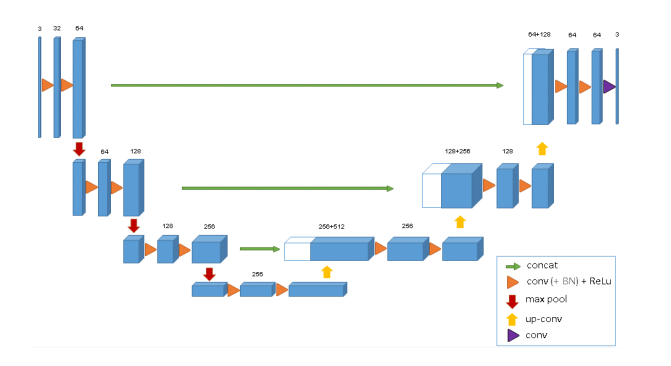
其中:
- 蓝色框表示的是特征图;
- 绿色长箭头,是
concat操作; - 橘色三角,是
conv+bn+relu的组合; - 红色的向下箭头,是
max pool; - 黄色的向上箭头,是
up conv; - 最后的紫色三角,是
conv,恢复了最终的输出特征图;
对于模型构建这块,可以在论文中,看看作者是如何描述网络结构的:
Like the standard u-net, it has an analysis and a synthesis path each with four resolution steps.In the analysis path, each layer contains two 3 × 3 × 3 convolutions each followed by a rectified linear unit (ReLu), and then a 2 × 2 × 2 max pooling with strides of two in each dimension.In the synthesis path, each layer consists of an upconvolution of 2 × 2 × 2 by strides of two in each dimension, followed by two 3 × 3 × 3 convolutions each followed by a ReLu.Shortcut connections from layers of equal resolution in the analysis path provide the essential high-resolution features to the synthesis path.In the last layer a 1×1×1 convolution reduces the number of output channels to the number of labels which is 3 in our case.
从论文中的网络结构示意图也可以发现:
- 水平看,每一个小块,基本都是三个特征图,最后一层除外;
- 水平看,每个特征图之间,都是橘色三角,是
conv+bn+relu的组合,最后一层除外; encoder阶段,连接各个水平块的,是下采样;decoder阶段,连接各个水平块的,是反卷积(upconvolution);- 还有就是绿色长箭头的
concat,和最后的conv输出特征图。
二、 3D UNet 复现
复线在
3D UNet前,可以先参照下相对简单,且很深渊源的2D UNet结构。其中被多次使用的一个水平块中,也是两个conv+bn+relu的组合,2D UNet的构建如下所示:class ConvBlock2d(nn.Module): def __init__(self, in_ch, out_ch): super(ConvBlock2d, self).__init__() # 第1个3*3的卷积层 self.conv1 = nn.Sequential( nn.Conv2d(in_ch, out_ch, kernel_size=3, stride=1, padding=1), nn.BatchNorm2d(out_ch), nn.ReLU(inplace=True), ) # 第2个3*3的卷积层 self.conv2 = nn.Sequential( nn.Conv2d(out_ch, out_ch, kernel_size=3, stride=1, padding=1), nn.BatchNorm2d(out_ch), nn.ReLU(inplace=True), ) # 定义数据前向流动形式 def forward(self, x): x = self.conv1(x) x = self.conv2(x) return x- 1
- 2
- 3
- 4
- 5
- 6
- 7
- 8
- 9
- 10
- 11
- 12
- 13
- 14
- 15
- 16
- 17
- 18
- 19
- 20
- 21
- 22
- 23
而在
3D UNet的一个水平块中,同样是两个conv+bn+relu的组合,如下所示:is_elu = False def activateELU(is_elu, nchan): if is_elu: return nn.ELU(inplace=True) else: return nn.PReLU(nchan) def ConvBnActivate(in_channels, middle_channels, out_channels): # This is a block with 2 convolutions # The first convolution goes from in_channels to middle_channels feature maps # The second convolution goes from middle_channels to out_channels feature maps conv = nn.Sequential( nn.Conv3d(in_channels, middle_channels, stride=1, kernel_size=3, padding=1), nn.BatchNorm3d(middle_channels), activateELU(is_elu, middle_channels), nn.Conv3d(middle_channels, out_channels, stride=1, kernel_size=3, padding=1), nn.BatchNorm3d(out_channels), activateELU(is_elu, out_channels), ) return conv- 1
- 2
- 3
- 4
- 5
- 6
- 7
- 8
- 9
- 10
- 11
- 12
- 13
- 14
- 15
- 16
- 17
- 18
- 19
- 20
- 21
2.1、模块搭建
可以发现,
nn.Conv2d变成了nn.Conv3d,nn.BatchNorm2d变成了nn.BatchNorm3d。遵照这个规则,构建下采样MaxPool3d、上采样反卷积ConvTranspose3d,以及最后紫色一层卷积,输出特征层FinalConvolution,如下:def DownSample(): # It halves the spatial dimensions on every axes (x,y,z) return nn.MaxPool3d(kernel_size=2, stride=2) def UpSample(in_channels, out_channels): # It doubles the spatial dimensions on every axes (x,y,z) return nn.ConvTranspose3d(in_channels, out_channels, kernel_size=2, stride=2) def FinalConvolution(in_channels, out_channels): return nn.Conv3d(in_channels, out_channels, kernel_size=1)- 1
- 2
- 3
- 4
- 5
- 6
- 7
- 8
- 9
- 10
除此之外,绿色长箭头,
concat操作,是在水平方向上,也就是列上进行组合,如下所示:def CatBlock(x1, x2): return torch.cat((x1, x2), 1)- 1
- 2
至此,构建模型所需要的各个组块,都准备完毕了。接下来就是构建模型,将各个组块搭起来。其中有个规律:
- 除
encoder中第一conv+bn+relu外,每一次前都需要下采样; decoder中,每一个conv+bn+relu前,都需要上采样;- 并且,
decoder中第一个conv操作,需要进行concat操作; DownSample的channel不变,特征图尺寸变小;UpSample的channel不变,特征图尺寸变大;
那就把这些规则,根据图示给加上,组合后的一个类,就如下所示:
class UNet3D(nn.Module): def __init__(self, num_out_classes=2, input_channels=1, init_feat_channels=32, testing=False): super().__init__() self.testing = testing # Encoder layers definitions self.down_sample = DownSample() self.init_conv = ConvBnActivate(input_channels, init_feat_channels, init_feat_channels*2) self.down_conv1 = ConvBnActivate(init_feat_channels*2, init_feat_channels*2, init_feat_channels*4) self.down_conv2 = ConvBnActivate(init_feat_channels*4, init_feat_channels*4, init_feat_channels*8) self.down_conv3 = ConvBnActivate(init_feat_channels*8, init_feat_channels*8, init_feat_channels*16) # Decoder layers definitions self.up_sample1 = UpSample(init_feat_channels*16, init_feat_channels*16) self.up_conv1 = ConvBnActivate(init_feat_channels*(16+8), init_feat_channels*8, init_feat_channels*8) self.up_sample2 = UpSample(init_feat_channels*8, init_feat_channels*8) self.up_conv2 = ConvBnActivate(init_feat_channels*(8+4), init_feat_channels*4, init_feat_channels*4) self.up_sample3 = UpSample(init_feat_channels*4, init_feat_channels*4) self.up_conv3 = ConvBnActivate(init_feat_channels*(4+2), init_feat_channels*2, init_feat_channels*2) self.final_conv = FinalConvolution(init_feat_channels*2, num_out_classes) # Softmax self.softmax = nn.Softmax(dim=1) # 多分类问题用soft-max函数作为输出 self.sigmoid = nn.Sigmoid() # 二分类问题用sigmoid函数作为输出,二分类下和softmax等价 def forward(self, image): # Encoder Part # # B x 1 x Z x Y x X layer_init = self.init_conv(image) # B x 64 x Z x Y x X max_pool1 = self.down_sample(layer_init) # B x 64 x Z//2 x Y//2 x X//2 layer_down2 = self.down_conv1(max_pool1) # B x 128 x Z//2 x Y//2 x X//2 max_pool2 = self.down_sample(layer_down2) # B x 128 x Z//4 x Y//4 x X//4 layer_down3 = self.down_conv2(max_pool2) # B x 256 x Z//4 x Y//4 x X//4 max_pool_3 = self.down_sample(layer_down3) # B x 256 x Z//8 x Y//8 x X//8 layer_down4 = self.down_conv3(max_pool_3) # B x 512 x Z//8 x Y//8 x X//8 # Decoder part # layer_up1 = self.up_sample1(layer_down4) # B x 512 x Z//4 x Y//4 x X//4 cat_block1 = CatBlock(layer_down3, layer_up1) # B x (256+512) x Z//4 x Y//4 x X//4 layer_conv_up1 = self.up_conv1(cat_block1) # B x 256 x Z//4 x Y//4 x X//4 layer_up2 = self.up_sample2(layer_conv_up1) # B x 256 x Z//2 x Y//2 x X//2 cat_block2 = CatBlock(layer_down2, layer_up2) # B x (128+256) x Z//2 x Y//2 x X//2 layer_conv_up2 = self.up_conv2(cat_block2) # B x 128 x Z//2 x Y//2 x X//2 layer_up3 = self.up_sample3(layer_conv_up2) # B x 128 x Z x Y x X cat_block3 = CatBlock(layer_init, layer_up3) # B x (64+128) x Z x Y x X layer_conv_up3 = self.up_conv3(cat_block3) # B x 64 x Z x Y x X final_layer = self.final_conv(layer_conv_up3) # B x 2 x Z x Y x X if self.testing: final_layer = self.sigmoid(final_layer) return final_layer- 1
- 2
- 3
- 4
- 5
- 6
- 7
- 8
- 9
- 10
- 11
- 12
- 13
- 14
- 15
- 16
- 17
- 18
- 19
- 20
- 21
- 22
- 23
- 24
- 25
- 26
- 27
- 28
- 29
- 30
- 31
- 32
- 33
- 34
- 35
- 36
- 37
- 38
- 39
- 40
- 41
- 42
- 43
- 44
- 45
- 46
- 47
- 48
- 49
- 50
- 51
- 52
- 53
- 54
- 55
- 56
- 57
- 58
- 59
- 60
- 61
- 62
- 63
- 64
- 65
- 66
- 67
- 68
- 69
- 70
- 71
- 72
- 73
- 74
- 75
- 76
- 77
- 78
- 79
2.2、模型初测
定义好了模型还不算完,分阶段测试下构建的网络是不是和我们所预想的一样。我们给他一个输入,测试下是否与我们最初的想法是一致的,是否报错等等问题,如下这样:
DEVICE = torch.device("cuda" if torch.cuda.is_available() else "cpu") # 没gpu就用cpu print(DEVICE) # Tensors for 3D Image Processing in PyTorch # Batch x Channel x Z x Y x X # Batch size BY x Number of channels x (BY Z dim) x (BY Y dim) x (BY X dim) if __name__ == '__main__': from torchsummary import summary model = UNet3D(num_out_classes=3, input_channels=3, init_feat_channels=32) # print(model) summary(model, input_size=(3, 128, 128, 64), batch_size=-1, device='cpu')- 1
- 2
- 3
- 4
- 5
- 6
- 7
- 8
- 9
- 10
- 11
- 12
- 13
打印的内容如下:
---------------------------------------------------------------- Layer (type) Output Shape Param # ================================================================ Conv3d-1 [-1, 32, 128, 128, 64] 2,624 BatchNorm3d-2 [-1, 32, 128, 128, 64] 64 PReLU-3 [-1, 32, 128, 128, 64] 32 Conv3d-4 [-1, 64, 128, 128, 64] 55,360 BatchNorm3d-5 [-1, 64, 128, 128, 64] 128 PReLU-6 [-1, 64, 128, 128, 64] 64 MaxPool3d-7 [-1, 64, 64, 64, 32] 0 Conv3d-8 [-1, 64, 64, 64, 32] 110,656 BatchNorm3d-9 [-1, 64, 64, 64, 32] 128 PReLU-10 [-1, 64, 64, 64, 32] 64 Conv3d-11 [-1, 128, 64, 64, 32] 221,312 BatchNorm3d-12 [-1, 128, 64, 64, 32] 256 PReLU-13 [-1, 128, 64, 64, 32] 128 MaxPool3d-14 [-1, 128, 32, 32, 16] 0 Conv3d-15 [-1, 128, 32, 32, 16] 442,496 BatchNorm3d-16 [-1, 128, 32, 32, 16] 256 PReLU-17 [-1, 128, 32, 32, 16] 128 Conv3d-18 [-1, 256, 32, 32, 16] 884,992 BatchNorm3d-19 [-1, 256, 32, 32, 16] 512 PReLU-20 [-1, 256, 32, 32, 16] 256 MaxPool3d-21 [-1, 256, 16, 16, 8] 0 Conv3d-22 [-1, 256, 16, 16, 8] 1,769,728 BatchNorm3d-23 [-1, 256, 16, 16, 8] 512 PReLU-24 [-1, 256, 16, 16, 8] 256 Conv3d-25 [-1, 512, 16, 16, 8] 3,539,456 BatchNorm3d-26 [-1, 512, 16, 16, 8] 1,024 PReLU-27 [-1, 512, 16, 16, 8] 512 ConvTranspose3d-28 [-1, 512, 32, 32, 16] 2,097,664 Conv3d-29 [-1, 256, 32, 32, 16] 5,308,672 BatchNorm3d-30 [-1, 256, 32, 32, 16] 512 PReLU-31 [-1, 256, 32, 32, 16] 256 Conv3d-32 [-1, 256, 32, 32, 16] 1,769,728 BatchNorm3d-33 [-1, 256, 32, 32, 16] 512 PReLU-34 [-1, 256, 32, 32, 16] 256 ConvTranspose3d-35 [-1, 256, 64, 64, 32] 524,544 Conv3d-36 [-1, 128, 64, 64, 32] 1,327,232 BatchNorm3d-37 [-1, 128, 64, 64, 32] 256 PReLU-38 [-1, 128, 64, 64, 32] 128 Conv3d-39 [-1, 128, 64, 64, 32] 442,496 BatchNorm3d-40 [-1, 128, 64, 64, 32] 256 PReLU-41 [-1, 128, 64, 64, 32] 128 ConvTranspose3d-42 [-1, 128, 128, 128, 64] 131,200 Conv3d-43 [-1, 64, 128, 128, 64] 331,840 BatchNorm3d-44 [-1, 64, 128, 128, 64] 128 PReLU-45 [-1, 64, 128, 128, 64] 64 Conv3d-46 [-1, 64, 128, 128, 64] 110,656 BatchNorm3d-47 [-1, 64, 128, 128, 64] 128 PReLU-48 [-1, 64, 128, 128, 64] 64 Conv3d-49 [-1, 3, 128, 128, 64] 195 ================================================================ Total params: 19,077,859 Trainable params: 19,077,859 Non-trainable params: 0 ---------------------------------------------------------------- Input size (MB): 12.00 Forward/backward pass size (MB): 8544.00 Params size (MB): 72.78 Estimated Total Size (MB): 8628.78 ----------------------------------------------------------------- 1
- 2
- 3
- 4
- 5
- 6
- 7
- 8
- 9
- 10
- 11
- 12
- 13
- 14
- 15
- 16
- 17
- 18
- 19
- 20
- 21
- 22
- 23
- 24
- 25
- 26
- 27
- 28
- 29
- 30
- 31
- 32
- 33
- 34
- 35
- 36
- 37
- 38
- 39
- 40
- 41
- 42
- 43
- 44
- 45
- 46
- 47
- 48
- 49
- 50
- 51
- 52
- 53
- 54
- 55
- 56
- 57
- 58
- 59
- 60
- 61
- 62
其中,我们测试的参数量是
19,077,859,论文中说的参数量:The architecture has 19069955 parameters in total.有略微的差别。后面再调用模型,进行一次前向传播,
loss运算和反向回归。如果这里都通过了,那么后面构建训练代码,就更简单了很多。如下:if __name__ == '__main__': input_channels = 3 num_out_classes = 2 init_feat_channels = 32 batch_size = 4 model = UNet3D(num_out_classes=num_out_classes, input_channels=input_channels, init_feat_channels=init_feat_channels) # B x C x Z x Y x X # 4 x 1 x 64 x 64 x 64 input_batch_size = (batch_size, input_channels, 128, 128, 64) input_example = torch.rand(input_batch_size) unet = model.to(DEVICE) input_example = input_example.to(DEVICE) output = unet(input_example) # output = output.cpu().detach().numpy() # Expected output shape # B x N x Z x Y x X # 4 x 2 x 64 x 64 x 64 expected_output_shape = (batch_size, num_out_classes, 128, 128, 64) print("Output shape = {}".format(output.shape)) assert output.shape == expected_output_shape, "Unexpected output shape, check the architecture!" expected_gt_shape = (batch_size, 128, 128, 64) ground_truth = torch.ones(expected_gt_shape) ground_truth = ground_truth.long().to(DEVICE) # Defining loss fn ce_layer = torch.nn.CrossEntropyLoss() # Calculating loss ce_loss = ce_layer(output, ground_truth) print("CE Loss = {}".format(ce_loss)) # Back propagation ce_loss.backward()- 1
- 2
- 3
- 4
- 5
- 6
- 7
- 8
- 9
- 10
- 11
- 12
- 13
- 14
- 15
- 16
- 17
- 18
- 19
- 20
- 21
- 22
- 23
- 24
- 25
- 26
- 27
- 28
- 29
- 30
- 31
- 32
- 33
- 34
- 35
- 36
输出内容如下:
Output shape = torch.Size([4, 2, 128, 128, 64]) CE Loss = 0.6823387145996094- 1
- 2
2.3、疑问汇总
在
GitHub上,一篇关于3D UNet的仓库,获得了1.6k 星星。链接地址在这里:pytorch-3dunet在这个
GitHub里面,增加了很多的注释,也带来了一些心中的疑惑。2.3.1、什么时候使用
softmax?什么时候使用sigmoid?选择使用
softmax或sigmoid作为输出层的依据取决于您的任务类型和具体情况。-
如果您的任务是对每个像素进行多类别分类(语义分割),例如图像分割任务,那么您可以使用
softmax作为输出层。softmax将为每个像素分配一个概率分布,表示该像素属于每个类别的概率,这样可以确保每个像素的预测结果归一化,并且所有通道的概率之和为1。这种方法通常用于分割器官或病变等结构。 -
如果您的任务是对每个像素进行二元分类,例如肿瘤检测任务,那么您可以使用
sigmoid作为输出层。sigmoid将为每个像素分配一个0到1之间的值,表示该像素属于正类的概率。这种方法通常用于检测二元结构,如肿瘤。但是,二元分类任务,使用softmax也是可以的。
总之,选择哪种输出层取决于您的任务类型和具体情况。
2.3.2、训练阶段是不需要
softmax/sigmoid?只在推理阶段使用呢?if True applies the final normalization layer (sigmoid or softmax), otherwise the networks returns the output from the final convolution layer; use False for regression problems, e.g. de-noising
-
在训练阶段,输出层的特征图通常不需要经过
sigmoid或softmax函数处理,因为在计算损失函数时,通常会使用原始的特征图和标签图进行比较。 -
在推理阶段,输出层的特征图需要经过
sigmoid或softmax函数处理,以将特征图转换为像素级别的预测结果。对于分割一个类别的任务,您可以使用sigmoid函数将特征图转换为像素级别的二进制掩码,表示每个像素属于结节的概率。对于分割多个类别的任务,您可以使用softmax函数将特征图转换为像素级别的类别标签。
因此,在推理阶段,您需要将输出层的特征图通过
sigmoid或softmax函数进行处理,以获得像素级别的预测结果。在上面的GitHub有个训练的提示,如下这样:
-
Training loss shape of target
- When training with binary-based losses, i.e.: BCEWithLogitsLoss, DiceLoss, BCEDiceLoss, GeneralizedDiceLoss: The
target data has to be 4D(one target binary mask per channel). - When training with WeightedCrossEntropyLoss, CrossEntropyLoss, PixelWiseCrossEntropyLoss the
target dataset has to be 3D, see also pytorch documentation for CE loss: https://pytorch.org/docs/master/generated/torch.nn.CrossEntropyLoss.html
- When training with binary-based losses, i.e.: BCEWithLogitsLoss, DiceLoss, BCEDiceLoss, GeneralizedDiceLoss: The
-
final_sigmoid in the model config section applies only to the inference time (validation, test):
- When training with
BCEWithLogitsLoss, DiceLoss, BCEDiceLoss, GeneralizedDiceLosssetfinal_sigmoid=True; - When training with cross entropy based losses (
WeightedCrossEntropyLoss, CrossEntropyLoss, PixelWiseCrossEntropyLoss) setfinal_sigmoid=False,so that Softmax normalization is applied to the output.
- When training with
2.3.3、在训练阶段,真的不可以加入sigmoid或softmax吗?
万事没有一个太绝对了。在训练阶段使用了
sigmoid或softmax也是可以的,以获得类似于推理阶段的预测结果。这种方法称为“软标签”,可以帮助模型更好地学习特征和提高分割结果的质量。(因为sigmoid或softmax类似于一个规范化层,可以降低提高收敛效率)使用软标签时,您需要将每个像素的标签从硬标签(0或1)转换为概率分布。对于分割一个类别的任务,您可以使用
sigmoid函数将标签转换为0到1之间的值,表示该像素属于结节的概率。对于分割多个类别的任务,您可以使用softmax函数将标签转换为每个类别的概率分布。请注意,使用软标签会增加模型的训练难度和计算复杂度。因此,
- 如果您的数据集足够大且质量良好,您可以不使用软标签来训练模型,也就是训练阶段不使用
sigmoid或softmax; - 但是如果您的数据集较小或存在噪声数据,使用软标签可能会提高模型的性能和分割结果的质量。也就是训练阶段使用
sigmoid或softmax。
在论文:3D U-Net: Learning Dense Volumetric Segmentation from Sparse Annotation,论文中第
3.2章节介绍了如何使用软标签。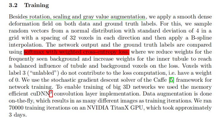
2.3.4、out_channels 的数量,要不要加背景层?
out_channels (int): number of output segmentation masks; Note that the of out_channels might correspond to either different semantic classes or to different binary segmentation mask.
It’s up to the user of the class to interpret the out_channels and use the proper loss criterion during training (i.e. CrossEntropyLoss (multi-class) or BCEWithLogitsLoss (two-class) respectively)我的理解是,有多少个目标类,
out_channels就是多少,不需要加背景类。但是,我也看到就只有一个类别,但是做了加1操作的。这点我再了解下。如果你有什么心得,欢迎评论区交流。三、总结
UNet网络的结构,无论是二维的,还是三维的,都是比较容易理解的,这可能也是为什么那么受欢迎的原因之一吧。如果你看过之前那篇关于2D UNet的过程,再看本篇应该就简单的很多。觉得本篇更简单一些呢。我觉得本篇最大的价值,就是:
- 逐模块的分析了结构;
- 对后续的模型构建提供了思路;
- 构建完模型需要先预测试,两种方式可选;
- 对模型的优势和劣势,分析。
如果你阅读的过程中,发现了问题和疑问,欢迎评论区交流。
最后,如果您觉得本篇文章对你有帮助,欢迎点赞 👍,让更多人看到,这是对我继续写下去的鼓励。如果能再点击下方的红包打赏,给博主来一杯咖啡,那就太好了。💪
-
相关阅读:
CSS|02 基本选择器
深入理解c++继承
高保真神经网络音频编码器
第58章 结构、纪录与类
Xilinx 高速AD 设计参考(在网上找到的总结)
Acrobat Pro DC 2021:强大的PDF编辑软件
QT调用百度地图并返回点击地的经纬度
Oracle物化视图(Materialized View)
python自动化测试 namp端口扫描
【localStorage的理解与使用】
- 原文地址:https://blog.csdn.net/wsLJQian/article/details/134059062