一篇文章入门LSTM和GRU

NLP

长短期记忆神经网络（LSTM）

1、Recurrent Neural Networks

人类不会每秒钟都从头开始思考。当你阅读这篇文章时，你会根据你对前面单词的理解来理解每个单词。你不会把所有东西都扔掉，然后重新从头开始思考，你的思想有持久性。

传统的神经网络无法做到这一点，这似乎是一个主要缺点。循环神经网络解决了这个问题，它们是带有循环的网络，允许信息持续存在。

这些循环使循环神经网络看起来有点神秘。然而，如果你再想一想，就会发现它们与普通的神经网络并没有什么不同。循环神经网络可以被认为是同一网络的多个副本，每个副本都将消息传递给后继者。考虑一下如果我们展开循环会发生什么：

长期依赖问题

有时，我们只需要查看最近的信息即可执行当前任务。例如，考虑一个语言模型试图根据之前的单词预测下一个单词。如果我们试图预测“云在天空”中的最后一个词，我们不需要任何进一步的上下文——很明显下一个词将是天空。在这种情况下，相关信息与所需位置之间的差距很小，RNN 可以学习使用过去的信息。

但也有我们需要更多上下文的情况。考虑尝试预测文本“I grew up in France… I speak fluent French.”中的最后一个词。最近的信息表明，下一个词可能是一种语言的名称，但如果我们想缩小哪种语言的范围，我们需要从从更远的地方获得法国的上下文。相关信息与需要的点之间的差距完全有可能变得非常大。

不幸的是，随着差距的扩大，RNN 变得无法学习连接信息。

从理论上讲，RNN 绝对有能力处理这种“长期依赖”。人类可以为他们仔细挑选参数来解决这种形式的toy problem。遗憾的是，在实践中，RNN 似乎无法学习它们。

2、LSTM Networks

长短期记忆网络——通常称为“LSTM”——是一种特殊的 RNN，能够学习长期依赖关系。

LSTM 被明确设计为避免长期依赖问题。长时间记住信息实际上是他们的default behavior，而不是他们难以学习的东西！

所有循环神经网络都具有神经网络的重复模块链的形式。在标准 RNN 中，此重复模块将具有非常简单的结构，例如单个 tanh 层。

The repeating module in a standard RNN contains a single layer.

LSTM 也有这种链状结构，但重复模块有不同的结构。不是只有一个神经网络层，而是有四个，以一种非常特殊的方式进行交互。

The repeating module in an LSTM contains four interacting layers.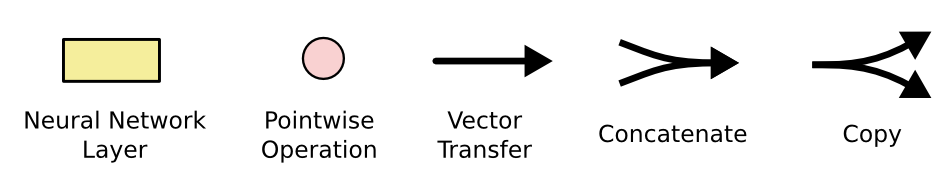

在上图中，每一行都携带一个完整的向量，从一个节点的输出到其他节点的输入。粉红色的圆圈代表逐点操作；如向量加法，而黄色的方框是学习的神经网络层；行合并表示连接；而行分叉表示其内容被复制并且副本到达不同的位置。

The Core Idea Behind LSTMs

LSTM 的关键是cell state，即贯穿图表顶部的水平线。

cell state有点像传送带。它直接沿着整个链条运行，只有一些较小的线性相互作用。信息很容易沿着它不变地流动。

LSTM 确实有能力将信息删除或添加到细胞状态，由称为gate的结构仔细调节。

gate是一种选择性地让信息通过的方式，它们由 sigmoid 神经网络层和pointwise multiplication operation组成。

sigmoid 层输出 0 到 1 之间的数字，表示让cell中的内容通过多少，值 0 表示“不让任何东西通过”，而值 1 表示“让所有东西通过！”

LSTM 具有其中三个门，用于保护和控制cell state

Step-by-Step LSTM Walk Through

我们 LSTM 的第一步是决定我们将从cell state中丢弃哪些信息（我们之所以既可以记住小时候的事情，也可以记住一年前的事情，也没有觉得脑子不够用，是因为我们爱忘事），这个决定是由一个称为“遗忘门层”的 sigmoid 层做出的。

让我们回到我们的语言模型示例，该示例试图根据所有先前的单词来预测下一个单词。在这样的问题中，cell state可能包括当前主语的性别，因此可以使用正确的代词。当我们看到一个新主语时，我们想忘记旧主语的性别。

下一步是决定我们将在cell state中存储哪些新信息（只记忆该记忆的信息，我们在生活中也只能长久地记住很少的信息，大部分信息没过几天就忘了），这有两个部分：首先输入门将决定我们将要更新哪些值；接下来，使用tanh激活函数创建一个新的候选值向量，该候选值向量将被添加到cell state中

在我们的语言模型示例中，我们希望将新新主语的性别添加到cell state中，以替换我们忘记的旧主语。

现在是时候将旧的cell stateC_t-1更新为新的cell stateC_t

在语言模型的情况下，正如我们在前面的步骤中决定的那样，我们实际上会在此处删除有关旧主语性别的信息并添加新信息。

最后，我们需要决定要输出什么（假如我们每个脑细胞都只记一件事情，当我们在处理眼前的事情的时候我们只会调动和当前事情有关的脑细胞）。此输出将基于我们的cell state，但将是过滤后的版本。首先，我们运行一个 sigmoid 层，它决定我们要将cell state中的哪些状态进行输出。然后，我们将cell state通过tanh激活函数并将其乘以forget gate，这样我们只输出我们决定输出的部分

Variants on Long Short Term Memory

peephole connections：

另一种变体是使用耦合的遗忘门和输入门，我们不将忘记cell state中的旧信息和向cell state中添加新信息分开，相反只有我们忘记旧的东西时我们才会向cell state中输入新的信息

Gated Recurrent Unit（GRU）：它将遗忘门和输入门组合成一个“更新门”。它还合并了cell state和hidden state，并进行了一些其他更改。生成的模型比标准LSTM模型更简单，并且越来越受欢迎。

3、GRU

LSTM 通过门控机制使循环神经网络不仅能记忆过去的信息，同时还能选择性地忘记一些不重要的信息而对长期语境等关系进行建模，而 GRU 基于这样的想法在保留长期序列信息下减少梯度消失问题。

GRU 旨在解决标准 RNN 中出现的梯度消失问题

GRU 背后的原理与 LSTM 非常相似，即用门控机制控制输入、记忆等信息而在当前时间步做出预测，表达式由以下给出：

GRU有两个门，即一个重置门（reset gate）和一个更新门（update gate）。从直观上来说，重置门决定了如何将新的输入信息与前面的记忆相结合，更新门定义了前面记忆和当前记忆保存到当前时间步的量。

GRU的输入输出结构

GRU的输入输出结构与普通的RNN是一样的。有一个当前的输入 x^t ，和上一个节点传递下来的隐状态（hidden state） h^t−1 ，这个隐状态包含了之前节点的相关信息。

结合 x^t 和 h^t-1，GRU会得到当前隐藏节点的输出 y^t 和传递给下一个节点的隐状态 h^t 。

GRU的内部结构

首先，我们先通过上一个传输下来的状态 h^t-1和当前节点的输入 x^t 来获取两个门控状态。其中 r 控制重置的门控（reset gate）， z 为控制更新的门控（update gate）。

得到门控信号之后，首先使用重置门控来得到“重置”之后的数据：
，再将 h^t−1′ 与输入 x^t 进行拼接，再通过一个tanh激活函数来将数据放缩到-1~1的范围内

这里的 h′ 主要是包含了当前输入的 x^t 数据。有针对性地对 h′ 添加到当前的隐藏状态，相当于”记忆了当前时刻的状态“

⊙ 是Hadamard Product，也就是操作矩阵中对应的元素相乘，因此要求两个相乘矩阵是同型的；⊕ 则代表进行矩阵加法操作

**”更新记忆“**阶段：在这个阶段，我们同时进行了遗忘了记忆两个步骤。我们使用了先前得到的更新门控 z （update gate）

更新表达式：

门控信号（这里的 z ）的范围为0~1。门控信号越接近1，代表”记忆“下来的数据越多；而越接近0则代表”遗忘“的越少。（这一步的操作就是忘记传递下来的 h^t−1 中的某些维度信息，并加入当前节点输入的某些维度信息。）

这里的遗忘 (1-z) 和选择 z 是联动的。也就是说，对于传递进来的维度信息，我们会进行选择性遗忘，则遗忘了多少权重 （1-z ），我们就会使用包含当前输入的 h′ 中所对应的权重(1−z) 进行弥补。以保持一种”恒定“状态。

大家看到 r (reset gate)实际上与他的名字有点不符。我们仅仅使用它来获得了 h′ 。

那么这里的 h′ 实际上可以看成对应于LSTM中的hidden state；上一个节点传下来的 h^t−1 则对应于LSTM中的cell state。1-z对应的则是LSTM中的 forget gate，那么 z我们似乎就可以看成是输入门input gate。

GRU的原理

使用门控机制学习长期依赖关系的基本思想和 LSTM 一致，但还是有一些关键区别：

• GRU 有两个门（重置门与更新门），而 LSTM 有三个门（输入门、遗忘门和输出门）。
• GRU 并不会控制并保留内部记忆（c_t），且没有 LSTM 中的输出门。
• LSTM 中的输入与遗忘门对应于 GRU 的更新门，重置门直接作用于前面的隐藏状态。

为了解决标准 RNN 的梯度消失问题，GRU 使用了更新门（update gate）与重置门（reset gate）。基本上，这两个门控向量决定了哪些信息最终能作为门控循环单元的输出。这两个门控机制的特殊之处在于，它们能够保存长期序列中的信息，且不会随时间而清除或因为与预测不相关而移除。

首先我们需要指定以下符号：

更新门

在时间步 t，我们首先需要使用以下公式计算更新门 z_t：

其中 x_t 为第 t 个时间步的输入向量，即输入序列 X 的第 t 个分量，它会经过一个线性变换（与权重矩阵 W(z) 相乘）。h_(t-1) 保存的是前一个时间步 t-1 的信息，它同样也会经过一个线性变换。更新门将这两部分信息相加并投入到 Sigmoid 激活函数中，因此将激活结果压缩到 0 到 1 之间。以下是更新门在整个单元的位置与表示方法。

更新门帮助模型决定到底要将多少过去的信息传递到未来，或到底前一时间步和当前时间步的信息有多少是需要继续传递的。这一点非常强大，因为模型能决定从过去复制所有的信息以减少梯度消失的风险。

重置门

本质上来说，重置门主要决定了到底有多少过去的信息需要遗忘，我们可以使用以下表达式计算：

该表达式与更新门的表达式是一样的，只不过线性变换的参数和用处不一样而已。下图展示了该运算过程的表示方法

如前面更新门所述，h_(t-1) 和 x_t 先经过一个线性变换，再相加投入 Sigmoid 激活函数以输出激活值。

当前记忆内容

现在我们具体讨论一下这些门控到底如何影响最终的输出。在重置门的使用中，新的记忆内容将使用重置门储存过去相关的信息，它的计算表达式为：

计算重置门 r_t 与 Uh_(t-1) 的 Hadamard 乘积，即 r_t 与 Uh_(t-1) 的对应元素乘积。因为前面计算的重置门是一个由 0 到 1 组成的向量，它会衡量门控开启的大小。例如某个元素对应的门控值为 0，那么它就代表这个元素的信息完全被遗忘掉。该 Hadamard 乘积将确定所要保留与遗忘的以前信息。

将这两部分的计算结果相加再投入双曲正切激活函数中。该计算过程可表示为：

当前时间步的最终记忆

在最后一步，网络需要计算 h_t，该向量将保留当前单元的信息并传递到下一个单元中。在这个过程中，我们需要使用更新门，它决定了当前记忆内容 h’_t 和前一时间步 h_(t-1) 中需要收集的信息是什么。这一过程可以表示为：

z_t 为更新门的激活结果，它同样以门控的形式控制了信息的流入。z_t 与 h_(t-1) 的 Hadamard 乘积表示前一时间步保留到最终记忆的信息，该信息加上当前记忆保留至最终记忆的信息就等于最终门控循环单元输出的内容

以上表达式可以展示为：

门控循环单元不会随时间而清除以前的信息，它会保留相关的信息并传递到下一个单元，因此它利用全部信息而避免了梯度消失问题。

4、pytorch代码实现（LSTM）

import torch.nn as nn
import torch

lstm = nn.LSTM(10, 20, num_layers=2,bidirectional=True)

# text: [seq_length, batch_size, input_size]
text = torch.randn(5, 3, 10)  # seq_length=5, batch_size=3, input_size=10

# h_0: [num_layers * num_directions, batch_size, hidden_size]
h_0 = torch.randn(4, 3, 20)  # num_layers*num_directions=2, batch_size=3, hidden_size=20

# c_0: [num_layers * num_directions, batch_size, hidden_size]
c_0 = torch.randn(4, 3, 20)  # num_layers*num_directions=2, batch_size=3, hidden_size=20

output, (h_n, c_n) = lstm(text)

# output: [seq_length, batch_size, num_directions * hidden_size]
print(output.shape)  # seq_length=5, batch_size=3, num_directions * hidden_size=20

# h_n: [num_layers * num_directions, batch_size, hidden_size]
print(h_n.size())  # num_layers * num_directions=2, batch_size=3, hidden_size=20

# c_n: [num_layers * num_directions, batch_size, hidden_size]
print(c_n.shape)  # num_layers * num_directions=2, batch_size=3, hidden_size=20
1
2
3
4
5
6
7
8
9
10
11
12
13
14
15
16
17
18
19
20
21
22
23
24

import torch
import torch.nn as nn

batch_size = 10
seq_length = 20  # 句子的长度
dictionary_size = 100  # 词典中词语的数量
embedding_dim = 30  # 长度为30的向量表示一个词语
hidden_size = 18
num_layer = 2

# 构造一个batch的数据
text = torch.randint(low=0, high=100, size=[batch_size, seq_length])

print(text.shape)

# 数据经过embedding处理
embedding = nn.Embedding(dictionary_size, embedding_dim)
text_embedded = embedding(text)

# 传入LSTM
lstm = nn.LSTM(input_size=embedding_dim,
               hidden_size=hidden_size,
               num_layers=num_layer,
               batch_first=True)

'''
output: [batch_size, seq_length, num_directions * hidden_size]
h_n: [num_layers * num_directions, batch_size, hidden_size]
c_n: [num_layers * num_directions, batch_size, hidden_size]
'''
output, (h_n, c_n) = lstm(text_embedded)

# output把每一个时间步上的结果在seq_length这一维度上进行了拼接
print(output.shape)  # torch.Size([10, 20, 36])
print(f"{'*' * 20}")

# h_n把不同层的隐藏状态在第0个维度上进行了拼接
print(h_n.size())  # torch.Size([2, 10, 18])
print(f"{'*' * 20}")

print(c_n.shape)  # torch.Size([2, 10, 18])
print(f"{'*' * 20}")

# 最后一次的h_1应该和output的最后一个time step的输出是一样的

# 获取最后一个时间步上的输出
last_output = output[:, -1, :]

# 获取最后一次的hidden_state
last_hidden_state = h_n[-1, :, :]

print(last_output == last_hidden_state)
1
2
3
4
5
6
7
8
9
10
11
12
13
14
15
16
17
18
19
20
21
22
23
24
25
26
27
28
29
30
31
32
33
34
35
36
37
38
39
40
41
42
43
44
45
46
47
48
49
50
51
52

交叉熵损失：把softmax概率传入对数似然损失得到的损失函数称为交叉熵损失：

在pytorch中有两种方法实现交叉熵损失：

criterion=nn.CrossEntropyLoss()
loss=criterion(input, target)
1
2

# 1、对输出值计算softmax和取对数
output=F.log_softmax(x,dim=-1)
# 2、使用torch中带权损失
loss=F.nll_loss(output,target)
1
2
3
4

双向LSTM

单向的RNN，是根据前面的信息推出后面的，但是有时候只看前面的词是不够的，可能需要预测的词和后面的内容也相关，那么需要一种机制，能够让模型不仅能够从前往后的具有记忆，还需要从后往前的具有记忆，此时双向LSTM能够帮助我们解决这个问题

由于是双向LSTM，所以每个方向的LSTM都会有一个输出，最终的输出会有两部分，所以往往需要concat的操作

import torch
import torch.nn as nn

batch_size = 10
seq_length = 20  # 句子的长度
dictionary_size = 100  # 词典中词语的数量
embedding_dim = 30  # 长度为30的向量表示一个词语
hidden_size = 18
num_layer = 1

# 构造一个batch的数据
text = torch.randint(low=0, high=100, size=[batch_size, seq_length])

print(text.shape)
print(f"{'*' * 20}")

# 数据经过embedding处理
embedding = nn.Embedding(dictionary_size, embedding_dim)
text_embedded = embedding(text)

# 传入LSTM
lstm = nn.LSTM(input_size=embedding_dim,
               hidden_size=hidden_size,
               num_layers=num_layer,
               batch_first=True, bidirectional=True)

'''
output: [batch_size, seq_length, num_directions * hidden_size]
h_n: [num_layers * num_directions, batch_size, hidden_size]
c_n: [num_layers * num_directions, batch_size, hidden_size]
'''
output, (h_n, c_n) = lstm(text_embedded)

# output把每一个时间步上的结果在seq_length这一维度上进行了拼接
# 如果lstm是双向的，则output的num_directions * hidden_size维度中前面是前hidden_size个数据是正向lstm的输出，后hidden_size个数据是反向lstm的输出
print(output.shape)  # torch.Size([10, 20, 36])
print(f"{'*' * 20}")

# h_n把不同层的隐藏状态在第0个维度上进行了拼接
# h_n把双向lstm中正向的hidden_state和反向的hidden_state在第0个维度上也进行了拼接
print(h_n.size())  # torch.Size([2, 10, 18])
print(f"{'*' * 20}")

print(c_n.shape)  # torch.Size([2, 10, 18])
print(f"{'*' * 20}")

# 获取双向lstm中正向最后一个时间步的output
forward_output = output[:, -1, :18]
print(forward_output.shape)
print(f"{'*' * 20}")

# 获取双向lstm中正向的最后一个hidden_state
forward_h_n = h_n[-2, :, :]
print(forward_h_n.shape)
print(f"{'*' * 20}")

print(f"正向output和正向h_n是否相等：{forward_output == forward_h_n}")

# 获取双向lstm中反向最后一个时间步的output
backward_output = output[:, 0, 18:]
print(backward_output.shape)
print(f"{'*' * 20}")

# 获取双向lstm中反向的最后一个hidden_state
backward_h_n=h_n[-1,:,:]
print(backward_h_n.shape)
print(f"{'*' * 20}")

print(f"反向output和反向h_n是否相等：{backward_output == backward_h_n}")
1
2
3
4
5
6
7
8
9
10
11
12
13
14
15
16
17
18
19
20
21
22
23
24
25
26
27
28
29
30
31
32
33
34
35
36
37
38
39
40
41
42
43
44
45
46
47
48
49
50
51
52
53
54
55
56
57
58
59
60
61
62
63
64
65
66
67
68
69

import torch
import torch.nn as nn

batch_size = 10
seq_length = 20  # 句子的长度
dictionary_size = 100  # 词典中词语的数量
embedding_dim = 30  # 长度为30的向量表示一个词语
hidden_size = 18
num_layer = 2

# 构造一个batch的数据
text = torch.randint(low=0, high=100, size=[batch_size, seq_length])

print(text.shape)

# 数据经过embedding处理
embedding = nn.Embedding(dictionary_size, embedding_dim)
text_embedded = embedding(text)

# 传入LSTM
lstm = nn.LSTM(input_size=embedding_dim,
               hidden_size=hidden_size,
               num_layers=num_layer,
               batch_first=True)

'''
output: [batch_size, seq_length, num_directions * hidden_size]
h_n: [num_layers * num_directions, batch_size, hidden_size]
c_n: [num_layers * num_directions, batch_size, hidden_size]
'''
output, (h_n, c_n) = lstm(text_embedded)

# output把每一个时间步上的结果在seq_length这一维度上进行了拼接
print(output.shape)  # torch.Size([10, 20, 36])
print(f"{'*' * 20}")

# h_n把不同层的隐藏状态在第0个维度上进行了拼接
print(h_n.size())  # torch.Size([2, 10, 18])
print(f"{'*' * 20}")

print(c_n.shape)  # torch.Size([2, 10, 18])
print(f"{'*' * 20}")

# 最后一次的h_1应该和output的最后一个time step的输出是一样的

# 获取最后一个时间步上的输出
last_output = output[:, -1, :]

# 获取最后一次的hidden_state
last_hidden_state = h_n[-1, :, :]

'''
-4/1 第一层的正向
-3/2 第一层的反向
-2/3 第二层的正向
-1/4 第二层的反向
'''

print(last_output == last_hidden_state)
1
2
3
4
5
6
7
8
9
10
11
12
13
14
15
16
17
18
19
20
21
22
23
24
25
26
27
28
29
30
31
32
33
34
35
36
37
38
39
40
41
42
43
44
45
46
47
48
49
50
51
52
53
54
55
56
57
58
59

使用双向LSTM实现文本情感分类

import torch
import torch.nn as nn
import torch.nn.functional as F
from torch import optim
from dataset import get_dataloader
from pkl import ws, MAX_LEN
from datetime import datetime
from tqdm import tqdm

device = torch.device('cuda:0' if torch.cuda.is_available() else 'cpu')


class ImdbModule(nn.Module):
    def __init__(self, input_size, hidden_size, output_size):
        super(ImdbModule, self).__init__()

        self.embedding = nn.Embedding(len(ws), input_size, padding_idx=ws.PAD)

        self.hidden_size = hidden_size

        '''
        nn.LSTM:
            Args:
                input_size: The number of expected features in the input `x`
                hidden_size: The number of features in the hidden state `h`
                num_layers: Number of recurrent layers.
                bias: If `False`, then the layer does not use bias weights `b_ih` and `b_hh`.
                batch_first: If `True`, then the input and output tensors are provided as (batch, seq, feature).
                bidirectional: If `True`, becomes a bidirectional LSTM.
        '''

        '''
        input:
            x: [seq_length, batch_size, input_size] (tensor containing the features of the input sequence.)
            h_0: [num_layers * num_directions, batch_size, hidden_size] (tensor
              containing the initial hidden state for each element in the batch.)
            c_0: [num_layers * num_directions, batch_size, hidden_size] (tensor
              containing the initial cell state for each element in the batch.)
        return: output, (h_n, c_n):
            output: [seq_length, batch_size, num_directions * hidden_size]
            h_n: [num_layers * num_directions, batch_size, hidden_size]
            c_n: [num_layers * num_directions, batch_size, hidden_size]
        '''
        self.lstm = nn.LSTM(input_size=input_size,
                            hidden_size=self.hidden_size,
                            num_layers=2, bidirectional=True)

        self.linear = nn.Linear(2 * self.hidden_size, output_size)

    def forward(self, x):
        '''
        :param x: [batch_size, seq_length]
        :param h_0: [num_layers * num_directions, batch_size, hidden_size]
        :param c_0: [num_layers * num_directions, batch_size, hidden_size]
        :return:
        '''

        batch_size = x.size(0)

        # x: [batch_size, seq_length, input_size]
        x = self.embedding(x)

        # x: [seq_length, batch_size, input_size]
        x = x.permute(1, 0, 2)

        # output: [seq_length, batch_size, num_directions * hidden_size]
        # h_n: [num_layers * num_directions, batch_size, hidden_size]
        # c_n: [num_layers * num_directions, batch_size, hidden_size]
        output, (h_n, c_n) = self.lstm(x)

        # 往往会使用LSTM or GRU输出的最后一维结果来代表LSTM、GRU对文本处理的结果
        # 使用双向LSTM的时候，往往会使用每个方向最后一次的output，作为当前数据经过双向LSTM的结果

        out = torch.cat((h_n[-2, :, :], h_n[-1, :, :]), dim=-1)
        out = self.linear(out)

        return out


TRAIN_BATCH_SIZE = 128
TEST_BATCH_SIZE = 128
LR = 0.001

imdb = ImdbModule(100, 256, 11).to(device)

optimizer = optim.Adam(imdb.parameters(), lr=LR)

criterion = nn.CrossEntropyLoss().to(device)


def train_test(epoch):
    print(f"{'-' * 10}epoch: {epoch + 1}{'-' * 10}")

    mode = True
    imdb.train(mode)

    train_dataloader, train_data_length = get_dataloader(mode='train', batch_size=TRAIN_BATCH_SIZE)

    for idx, (text, label) in enumerate(train_dataloader):
        text = text.to(device)
        label = label.to(device)

        optimizer.zero_grad()

        # 第一次调用LSTM模型之前，需要初始化隐藏状态，如果不初始化，默认创建全为0的隐藏状态
        output = imdb(text)

        loss = criterion(output, label)

        loss.backward()
        optimizer.step()

        if idx % 50 == 0:
            print(f"第{epoch}轮训练次数为{idx}的误差：{loss.item()}")

    print(f"{'-' * 10}测试开始{'-' * 10}")

    imdb.eval()

    test_dataloader, len_test_data = get_dataloader('test', batch_size=TEST_BATCH_SIZE)

    sum_loss = 0
    total_accuracy = 0

    with torch.no_grad():
        for text, label in tqdm(test_dataloader):
            text = text.to(device)
            label = label.to(device)

            output = imdb(text)

            loss = criterion(output, label)
            sum_loss += loss

            predicted = output.argmax(1)
            accuracy = (predicted == label).sum()

            total_accuracy += accuracy

    print(f"测试集上的loss：{sum_loss}")

    correct_accuracy = total_accuracy / len_test_data
    print(f"整体测试集上的正确率：{correct_accuracy}%")

    print("模型保存成功")
    torch.save(imdb.state_dict(), f'./model/lstm_{epoch}.pth')

    now = datetime.now()
    now = now.strftime("%Y-%m-%d %H:%M:%S")

    content = f"time：{now}\tlstm模型在测试集上的准确率：{correct_accuracy}"

    with open('./accuracy.txt', 'a+', encoding='utf-8') as file:
        file.write(content + '\n')


for epoch in range(100):
    train_test(epoch)
1
2
3
4
5
6
7
8
9
10
11
12
13
14
15
16
17
18
19
20
21
22
23
24
25
26
27
28
29
30
31
32
33
34
35
36
37
38
39
40
41
42
43
44
45
46
47
48
49
50
51
52
53
54
55
56
57
58
59
60
61
62
63
64
65
66
67
68
69
70
71
72
73
74
75
76
77
78
79
80
81
82
83
84
85
86
87
88
89
90
91
92
93
94
95
96
97
98
99
100
101
102
103
104
105
106
107
108
109
110
111
112
113
114
115
116
117
118
119
120
121
122
123
124
125
126
127
128
129
130
131
132
133
134
135
136
137
138
139
140
141
142
143
144
145
146
147
148
149
150
151
152
153
154
155
156
157
158

5、pytorch代码实现（GRU）

import torch.nn as nn
import torch

'''
GRU:
    Applies a multi-layer gated recurrent unit (GRU) RNN to an input sequence.

    args:
        input_size: The number of expected features in the input `x`
        hidden_size: The number of features in the hidden state `h`
        num_layers: Number of recurrent layers.
        bias: If `False`, then the layer does not use bias weights
        bidirectional: If `True`, becomes a bidirectional GRU.
'''

'''
Inputs: input, h_0
    input: [seq_length, batch_size, input_size]
    h_0: [num_layers * num_directions, batch_size, hidden_size]

Outputs: output, h_n
    output: [seq_length, batch_size, num_directions * hidden_size]
    h_n: [num_layers * num_directions, batch_size, hidden_size]
'''
gru = nn.GRU(input_size=10, hidden_size=20, num_layers=2, bidirectional=True)

# text: [seq_length, batch_size, input_size]
text = torch.randn(5, 3, 10)

# h_0: [num_layers * num_directions, batch_size, hidden_size]
h_0 = torch.randn(4, 3, 20)

'''
output: [seq_length, batch_size, num_directions * hidden_size]
h_n: [num_layers * num_directions, batch_size, hidden_size]
'''
output, h_n = gru(text, h_0)

# 获取双向gru中正向最后一个时间步的output
forward_output=output[-1,:,:20]
print(forward_output.shape) # [batch_size, hidden_size]
print(f"{'*' * 20}")

# 获取双向gru中正向的最后一个hidden_state
forward_h_n=h_n[-2,:,:]
print(forward_h_n.shape) # [batch_size, hidden_size]
print(f"{'*' * 20}")

print(f"正向output和正向h_n是否相等：{forward_output == forward_h_n}")

# 获取双向gru中反向最后一个时间步的output
backward_output=output[0,:,20:]
print(backward_output.shape) # [batch_size, hidden_size]
print(f"{'*' * 20}")

# 获取双向gru中反向的最后一个hidden_state
backward_h_n=h_n[-1,:,:]
print(backward_h_n.shape)
print(f"{'*' * 20}")

print(f"反向output和反向h_n是否相等：{backward_output == backward_h_n}")
1
2
3
4
5
6
7
8
9
10
11
12
13
14
15
16
17
18
19
20
21
22
23
24
25
26
27
28
29
30
31
32
33
34
35
36
37
38
39
40
41
42
43
44
45
46
47
48
49
50
51
52
53
54
55
56
57
58
59
60
61

使用双向GRU实现文本情感分类

import torch
import torch.nn as nn
import torch.nn.functional as F
from torch import optim
from dataset import get_dataloader
from pkl import ws, MAX_LEN
from datetime import datetime
from tqdm import tqdm

device = torch.device('cuda:0' if torch.cuda.is_available() else 'cpu')


class ImdbModule(nn.Module):
    def __init__(self, input_size, hidden_size, output_size):
        super(ImdbModule, self).__init__()

        self.embedding = nn.Embedding(len(ws), input_size, padding_idx=ws.PAD)

        self.hidden_size = hidden_size

        '''
        GRU:
            Applies a multi-layer gated recurrent unit (GRU) RNN to an input sequence.
            
            args:
                input_size: The number of expected features in the input `x`
                hidden_size: The number of features in the hidden state `h`
                num_layers: Number of recurrent layers.
                bias: If `False`, then the layer does not use bias weights
                bidirectional: If `True`, becomes a bidirectional GRU.
        '''

        '''
        Inputs: input, h_0
            input: [seq_length, batch, input_size]
            h_0: [num_layers * num_directions, batch_size, hidden_size]
            
        Outputs: output, h_n
            output: [seq_length, batch_size, num_directions * hidden_size]
            h_n: [num_layers * num_directions, batch_size, hidden_size]
        '''

        self.gru = nn.GRU(input_size=input_size,
                          hidden_size=self.hidden_size,
                          num_layers=2,
                          bidirectional=True,
                          dropout=0.5)

        self.linear = nn.Linear(in_features=2 * hidden_size, out_features=output_size)
        self.dropout = nn.Dropout(0.5)

    def forward(self, x):
        '''
        :param x: [batch_size, seq_length]
        :return:
        '''

        batch_size = x.size(0)

        # x: [batch_size, seq_length, embedding_dim]
        x = self.embedding(x)

        # x: [seq_length, batch_size, input_size]
        x = x.permute(1, 0, 2)

        '''
        output: [seq_length, batch_size, num_directions * hidden_size]
        h_n: [num_layers * num_directions, batch_size, hidden_size]
        '''
        output, h_n = self.gru(x)

        h_n = torch.cat((h_n[-2, :, :], h_n[-1, :, :]), dim=-1)

        out = self.linear(h_n)

        return out


TRAIN_BATCH_SIZE = 128
TEST_BATCH_SIZE = 128
LR = 0.001

imdb = ImdbModule(256, 256, 11).to(device)

optimizer = optim.Adam(imdb.parameters(), lr=LR)

criterion = nn.CrossEntropyLoss().to(device)


def train_test(epoch):
    print(f"{'-' * 10}epoch: {epoch + 1}{'-' * 10}")

    mode = True
    imdb.train(mode)

    train_dataloader, train_data_length = get_dataloader(mode='train', batch_size=TRAIN_BATCH_SIZE)

    for idx, (text, label) in enumerate(train_dataloader):
        text = text.to(device)
        label = label.to(device)

        optimizer.zero_grad()

        # 第一次调用LSTM模型之前，需要初始化隐藏状态，如果不初始化，默认创建全为0的隐藏状态
        output = imdb(text)

        loss = criterion(output, label)

        loss.backward()
        optimizer.step()

        if idx % 50 == 0:
            print(f"第{epoch}轮训练次数为{idx}的误差：{loss.item()}")

    print(f"{'-' * 10}测试开始{'-' * 10}")

    imdb.eval()

    test_dataloader, len_test_data = get_dataloader('test', batch_size=TEST_BATCH_SIZE)

    sum_loss = 0
    total_accuracy = 0

    with torch.no_grad():
        for text, label in tqdm(test_dataloader):
            text = text.to(device)
            label = label.to(device)

            output = imdb(text)

            loss = criterion(output, label)
            sum_loss += loss

            predicted = output.argmax(1)
            accuracy = (predicted == label).sum()

            total_accuracy += accuracy

    print(f"测试集上的loss：{sum_loss}")

    correct_accuracy = total_accuracy / len_test_data
    print(f"整体测试集上的正确率：{correct_accuracy}%")

    print("模型保存成功")
    torch.save(imdb.state_dict(), f'./model/lstm_{epoch}.pth')

    now = datetime.now()
    now = now.strftime("%Y-%m-%d %H:%M:%S")

    content = f"time：{now}\tlstm模型在测试集上的准确率：{correct_accuracy}"

    with open('./accuracy.txt', 'a+', encoding='utf-8') as file:
        file.write(content + '\n')


for epoch in range(100):
    train_test(epoch)
1
2
3
4
5
6
7
8
9
10
11
12
13
14
15
16
17
18
19
20
21
22
23
24
25
26
27
28
29
30
31
32
33
34
35
36
37
38
39
40
41
42
43
44
45
46
47
48
49
50
51
52
53
54
55
56
57
58
59
60
61
62
63
64
65
66
67
68
69
70
71
72
73
74
75
76
77
78
79
80
81
82
83
84
85
86
87
88
89
90
91
92
93
94
95
96
97
98
99
100
101
102
103
104
105
106
107
108
109
110
111
112
113
114
115
116
117
118
119
120
121
122
123
124
125
126
127
128
129
130
131
132
133
134
135
136
137
138
139
140
141
142
143
144
145
146
147
148
149
150
151
152
153
154
155
156
157

相关前置内容和代码请参考：一篇文章入门循环神经网络RNN

参考

1、Understanding LSTM Networks

2、Understanding GRU Networks

3、人人都能看懂的GRU

4、Gated recurrent unit

5、阿达玛乘积 (矩阵)

6、关于Pytorch中双向LSTM的输出表示问题

7、[NLP自然语言处理]保姆级入门教程