Particle Swarm Optimization粒子群优化算法（PSO算法）概念及实战

Particle Swarm Optimization

粒子群算法（PSO算法）

定义

粒子群算法，又称粒子群优化算法（Particle Swarm Optimization），缩写为 PSO， 是近年来发展起来的一种新的进化算法（Evolutionary Algorithm - EA），由Eberhart 博士和Kennedy 博士于1995年提出，其源于对鸟群捕食的行为研究。

算法思想

PSO模拟鸟群的捕食行为。

设想这样一个场景：一群鸟在随机搜索食物，在这个区域里只有一块食物，所有的鸟都不知道食物在那里，但是它们知道当前的位置离食物还有多远，那么找到食物的最优策略是什么呢？

最简单有效的就是搜寻目前离食物最近的鸟的周围区域。都向这片区域靠拢。

抽象

PSO中，将问题的搜索空间类比于鸟类的飞行空间，将每只鸟抽象为一个无质量无体积的微粒，用以表征优化问题的一个候选解，我们称之为“粒子”，优化所需要寻找的最优解则等同于要寻找的食物。

所有的粒子都有一个由被优化的函数决定的适应值(fitness value)，每个粒子还有一个速度决定他们飞翔的方向和距离，然后粒子们就追随当前的最优粒子在解空间中搜索。

PSO初始化为一群随机粒子(随机解、一群鸟)，然后通过迭代找到最优解。在每一次迭代中，粒子（鸟）通过跟踪两个“极值”来更新自己的位置。一个就是粒子本身所找到的最优解，这个解叫做个体极值pBest，另一个极值是整个种群目前找到的最优解，这个极值是全局极值gBest。（gBest是pBest中最好值）

算法介绍

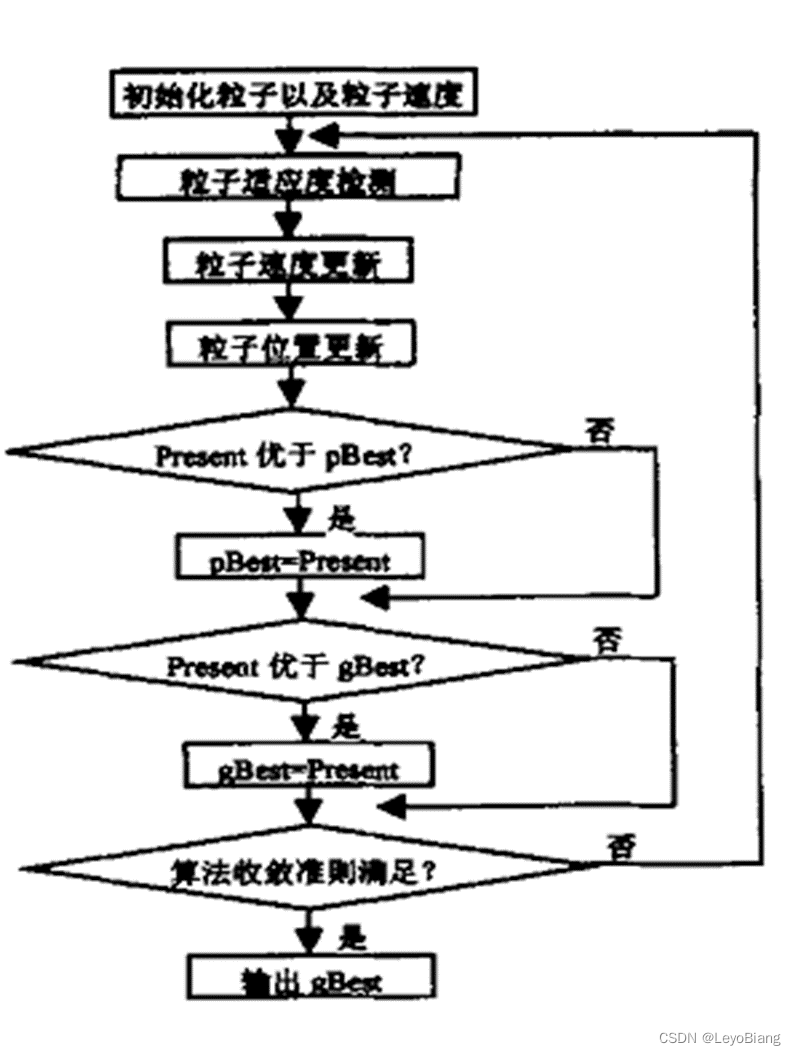
•在找到这两个最优值时，粒子根据如下的公式来更新自己的速度和位置：
$$\begin{gathered} V=w\times V \\ +c_1\times rand()\times (pBest-Present) \\ +c_2\times rand()\times (gBest-Present) \\ Present=Present+V \end{gathered}$$

• V 是例子速度 velocity
• Present 是粒子当前位置
• pBest 个体极值 最优解
• gBest 全局极值 最优解
• rand() 是(0,1)之间的随机数
• c_1、c_2 是学习因子 使粒子具有自我总结和向群体中优秀个体学习的能力，从而向群体内或邻域内最优点靠近，c_1和 c_2 通常等于2，并且范围在 0 和 4 之间
• w 是加权系数（惯性权重）决定了对粒子当前速度继承多少，合适的选择可以使粒子具有均衡的探索能力和开发能力，惯性权重的取法有常数法、线性递减法、自适应法等。
• Vmax: 最大速度，决定粒子在一个循环中最大的移动距离， 通常设定为粒子的范围宽度,例如，粒子 (x1, x2, x3) ，x1 属于 [-10, 10], 那么 x1的Vmax 的大小就是 20。
• 粒子数（鸟的个数）: 一般取 1~40. 其实对于大部分的问题10个粒子已经足够可以取得好的结果;
• 粒子的长度（维度）: 这是由优化问题决定, 就是问题解的长度（决策变量个数）;
• 粒子的范围: 由优化问题决定，每一维可以设定不同的范围；
• 中止条件: 最大循环数以及最小错误要求。

将粒子延伸到N维空间，粒子i在N维空间里的位置表示为一个矢量，每个粒子的飞行速度也表示为一个矢量。

举例

对于问题 f(x) = x1^2 + x2^2+x32 求解，粒子可以直接编码为 (x1, x2, x3)，而适应度函数就是f(x)，接着我们就可以利用前面的过程去寻优，寻优过程是一个迭代过程, 中止条件一般为设置为达到最大循环数或者最小错误要求。

例题

找下式的极大值
$$f(x,y)=\frac{sin\sqrt{x^2+y^2}}{\sqrt{x^2+y^2}}+e^{\frac{cos2\pi x+cos2\pi y}{2}}-2.71289$$

这里我们使用的工具是Python，我将从头到尾演示一下这整个过程

导入需要用的包

import random
import numpy as np
import math
import matplotlib.pyplot as plt
1
2
3
4

初始化粒子以及例子速度

这里我们选用了20个粒子，把粒子的x和y初始化在[-2,2]上，活动范围也都是[-2,2]，速度都是0，v_max设置为[10,10]

pBest我用来记录fitness value最大的位置，所以我先使pBest = particles，gBest 在这里取第一个pBest的值，如果一次迭代都没有的话那就会出错。

fxyRecord 用来记录每一轮迭代的fitness value的最大值，indexBest用来记录当前使fitness value最大的那个粒子的index

c1和c2学习因子都选用了2，w惯性权重选用了0.8

number_of_particles = 20
particles = np.random.rand(number_of_particles*2)*2
particles=particles.reshape((number_of_particles,2))
rangeParticle = np.array([[-2,2],[-2,2]])
velocities = np.zeros((number_of_particles, 2))
v_max = np.array([10,10])

pBest = particles.copy()
gBest = pBest[0]

fxyRecord = np.array([])
indexBest = 0

c1 = 2
c2 = 2
w = 0.8

epoch = 0
1
2
3
4
5
6
7
8
9
10
11
12
13
14
15
16
17
18

粒子适应度检测

首先我们要给出fitness value的计算函数

def f(x,y):
    sqrtx2plusy2 =math.sqrt(math.pow(x,2)+math.pow(y,2))
    firstTerm = math.sin(sqrtx2plusy2)/sqrtx2plusy2
    secondTerm  = math.exp((math.cos(2*math.pi*x) + math.cos(2*math.pi*y))/2)
    return firstTerm+secondTerm-2.71289
1
2
3
4
5

让每个粒子都计算出他当前的fitness value，并即使更新pBest和gBest，并用fxyRecord和indexBest记录其结果。

for index in range(number_of_particles):
    present = particles[index]
    x = present[0]
    y = present[1]
    fxy=f(x,y)
    if f(pBest[index][0],pBest[index][1]) < fxy:
        pBest[index] = np.array([x,y])
    if f(gBest[0],gBest[1]) < fxy:
        gBest =np.array([x,y])
        indexBest = index
fxyRecord=np.append(fxyRecord,f(gBest[0],gBest[1]))
1
2
3
4
5
6
7
8
9
10
11

粒子速度位置更新

根据当前的V、当前的位置（present）、pBest、gBest以及公式计算出下一个V，记得限制V的大小，然后保存这个计算出来的V作为当前的V

根据计算出的V 计算出下一个位置，同样需要限制粒子位置的范围（如果粒子的某个维度如果超过了range，在这里我设置这个粒子的这个维度的位置为被超过的这个range的值，这里其实还有各种各样的方案，比如反弹什么的，这个可以加入很多自己的畅想)，然后保存这个计算出来的位置作为当前的位置

for index in range(number_of_particles):
    present = particles[index]
    x = present[0]
    y = present[1]
    V = w*velocities[index] + c1*random.random()*(pBest[index]-present)+c2*random.random()*(gBest-present)

    # limit velocity
    if V[0]<v_max[0]*-1/2:
        V[0]=v_max[0]*-1/2
    elif V[0]>v_max[0]*1/2:
        V[0]=v_max[0]*1/2

    if V[1]<v_max[1]*-1/2:
        V[1]=v_max[1]*-1/2
    elif V[1]>v_max[1]*1/2:
        V[1]=v_max[1]*1/2
    velocities[index]=V
    
    particles[index]=present+V

    # limit coordinates
    if particles[index][0]<rangeParticle[0][0]:
        particles[index][0]=rangeParticle[0][0]
    elif particles[index][0]>rangeParticle[0][1]:
        particles[index][0]=rangeParticle[0][1]

    if particles[index][1]<rangeParticle[1][0]:
        particles[index][1]=rangeParticle[1][0]
    elif particles[index][1]>rangeParticle[1][1]:
        particles[index][1]=rangeParticle[1][1]
1
2
3
4
5
6
7
8
9
10
11
12
13
14
15
16
17
18
19
20
21
22
23
24
25
26
27
28
29
30

可视化

我通过绘制出粒子的位置以及迭代次数与fitness value对应的diagram来表现这个算法，使其相对直观一些，函数如下

def show(epoch):
    fig = plt.figure(figsize=(9,4))
    columns = 2
    rows = 1
    fig.add_subplot(rows, columns, 2)

    x_major_locator=plt.MultipleLocator(math.floor(epoch/10)+1)
    ax=plt.gca()
    ax.xaxis.set_major_locator(x_major_locator)
    plt.plot(fxyRecord)


    fig.add_subplot(rows, columns, 1)
    plt.xlim(np.array(gBest[0]+rangeParticle[0]/(epoch+1)))
    plt.ylim(np.array(gBest[1]+rangeParticle[1]/(epoch+1)))
    plt.scatter(particles.T[0],particles.T[1],s=10)
    plt.scatter(gBest[0],gBest[1],c='r',s=15)
1
2
3
4
5
6
7
8
9
10
11
12
13
14
15
16
17

尝试一下可视化

show(epoch)
epoch+=1
print(f"第{epoch}轮 极大值为:{f(gBest[0],gBest[1])} 对应粒子index:{indexBest} x:{gBest[0]} y:{gBest[1]}")
1
2
3

多运行几轮，逐一观察

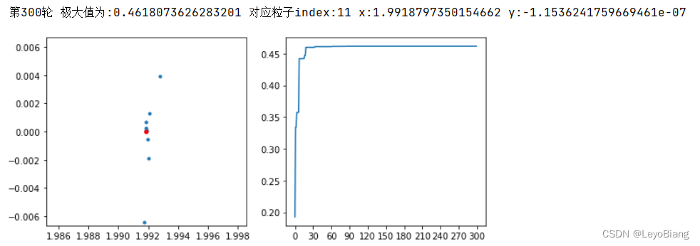
可见该算法还是相对容易陷入局部最优的问题，最好还是结合其他算法，来避免这个问题。

经过多次实验可以得到以下结果