《30天吃掉那只 TensorFlow2.0》 3-3 高阶API示范

3-3 高阶API示范

下面的范例使用TensorFlow的高阶API实现线性回归模型和DNN二分类模型。

TensorFlow的高阶API主要为tf.keras.models提供的模型的类接口。

使用Keras接口有以下3种方式构建模型：使用Sequential按层顺序构建模型，使用函数式API构建任意结构模型，继承Model基类构建自定义模型。

此处分别演示使用Sequential按层顺序构建模型以及继承Model基类构建自定义模型。

这里还是一开始定义一个打印时间分割线的函数

import tensorflow as tf

#打印时间分割线
@tf.function
def printbar():
    today_ts = tf.timestamp()%(24*60*60)

    hour = tf.cast(today_ts//3600+8,tf.int32)%tf.constant(24)
    minite = tf.cast((today_ts%3600)//60,tf.int32)
    second = tf.cast(tf.floor(today_ts%60),tf.int32)
    
    def timeformat(m):
        if tf.strings.length(tf.strings.format("{}",m))==1:
            return(tf.strings.format("0{}",m))
        else:
            return(tf.strings.format("{}",m))
    
    timestring = tf.strings.join([timeformat(hour),timeformat(minite),
                timeformat(second)],separator = ":")
    tf.print("=========="*8+timestring)

    
1
2
3
4
5
6
7
8
9
10
11
12
13
14
15
16
17
18
19
20
21
22

一，线性回归模型

此范例我们使用Sequential按层顺序构建模型，并使用内置model.fit方法训练模型【面向新手】。

1，准备数据

首先我们得先准备数据，我们可以用tensorflow来生成随机数，由于我们是线性回归，我们就可以利用矩阵乘法生成，并且加入一些正态扰动即可

import numpy as np 
import pandas as pd
from matplotlib import pyplot as plt 
import tensorflow as tf
from tensorflow.keras import models,layers,losses,metrics,optimizers

#样本数量
n = 400

# 生成测试用数据集
X = tf.random.uniform([n,2],minval=-10,maxval=10) 
w0 = tf.constant([[2.0],[-3.0]])
b0 = tf.constant([[3.0]])
Y = X@w0 + b0 + tf.random.normal([n,1],mean = 0.0,stddev= 2.0)  # @表示矩阵乘法,增加正态扰动

1
2
3
4
5
6
7
8
9
10
11
12
13
14
15

# 数据可视化

%matplotlib inline
%config InlineBackend.figure_format = 'svg'
plt.figure(figsize = (12,5))
ax1 = plt.subplot(121)
ax1.scatter(X[:,0],Y[:,0], c = "b")
plt.xlabel("x1")
plt.ylabel("y",rotation = 0)

ax2 = plt.subplot(122)
ax2.scatter(X[:,1],Y[:,0], c = "g")
plt.xlabel("x2")
plt.ylabel("y",rotation = 0)
plt.show()

1
2
3
4
5
6
7
8
9
10
11
12
13
14
15
16

2，定义模型

这里的定义模型，我们可以用tf.keras的高阶API，简单就可以定义完成，只需要通过add

tf.keras.backend.clear_session()

model = models.Sequential()
model.add(layers.Dense(1,input_shape =(2,)))
model.summary()
1
2
3
4
5

Model: "sequential"
_________________________________________________________________
Layer (type)                 Output Shape              Param #   
=================================================================
dense (Dense)                (None, 1)                 3         
=================================================================
Total params: 3
Trainable params: 3
Non-trainable params: 0
1
2
3
4
5
6
7
8
9

3，训练模型

这里可以直接用fit方法训练，不需要写过多的东西

### 使用fit方法进行训练

model.compile(optimizer="adam",loss="mse",metrics=["mae"])
model.fit(X,Y,batch_size = 10,epochs = 200)  

tf.print("w = ",model.layers[0].kernel)
tf.print("b = ",model.layers[0].bias)

1
2
3
4
5
6
7
8

Epoch 197/200
400/400 [==============================] - 0s 190us/sample - loss: 4.3977 - mae: 1.7129
Epoch 198/200
400/400 [==============================] - 0s 172us/sample - loss: 4.3918 - mae: 1.7117
Epoch 199/200
400/400 [==============================] - 0s 134us/sample - loss: 4.3861 - mae: 1.7106
Epoch 200/200
400/400 [==============================] - 0s 166us/sample - loss: 4.3786 - mae: 1.7092
w =  [[1.99339032]
 [-3.00866461]]
b =  [2.67018795]
1
2
3
4
5
6
7
8
9
10
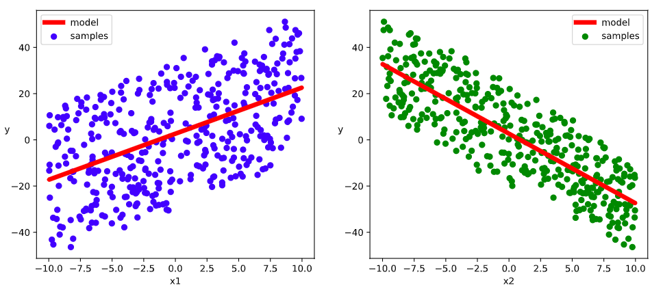
11

# 结果可视化

%matplotlib inline
%config InlineBackend.figure_format = 'svg'

w,b = model.variables

plt.figure(figsize = (12,5))
ax1 = plt.subplot(121)
ax1.scatter(X[:,0],Y[:,0], c = "b",label = "samples")
ax1.plot(X[:,0],w[0]*X[:,0]+b[0],"-r",linewidth = 5.0,label = "model")
ax1.legend()
plt.xlabel("x1")
plt.ylabel("y",rotation = 0)

ax2 = plt.subplot(122)
ax2.scatter(X[:,1],Y[:,0], c = "g",label = "samples")
ax2.plot(X[:,1],w[1]*X[:,1]+b[0],"-r",linewidth = 5.0,label = "model")
ax2.legend()
plt.xlabel("x2")
plt.ylabel("y",rotation = 0)

plt.show()
1
2
3
4
5
6
7
8
9
10
11
12
13
14
15
16
17
18
19
20
21
22
23

二，DNN二分类模型

此范例我们使用继承Model基类构建自定义模型，并构建自定义训练循环【面向专家】

1，准备数据

这里和前面有些类似，首先我们利用tensorflow的random函数来得到我们的数据

• 生成正样本, 小圆环分布

• 生成负样本, 大圆环分布

  生成后也可以可视化，对数据的分布有一个更好的理解

import numpy as np 
import pandas as pd 
from matplotlib import pyplot as plt
import tensorflow as tf
from tensorflow.keras import layers,losses,metrics,optimizers
%matplotlib inline
%config InlineBackend.figure_format = 'svg'

#正负样本数量
n_positive,n_negative = 2000,2000

#生成正样本, 小圆环分布
r_p = 5.0 + tf.random.truncated_normal([n_positive,1],0.0,1.0)
theta_p = tf.random.uniform([n_positive,1],0.0,2*np.pi) 
Xp = tf.concat([r_p*tf.cos(theta_p),r_p*tf.sin(theta_p)],axis = 1)
Yp = tf.ones_like(r_p)

#生成负样本, 大圆环分布
r_n = 8.0 + tf.random.truncated_normal([n_negative,1],0.0,1.0)
theta_n = tf.random.uniform([n_negative,1],0.0,2*np.pi) 
Xn = tf.concat([r_n*tf.cos(theta_n),r_n*tf.sin(theta_n)],axis = 1)
Yn = tf.zeros_like(r_n)

#汇总样本
X = tf.concat([Xp,Xn],axis = 0)
Y = tf.concat([Yp,Yn],axis = 0)

#样本洗牌
data = tf.concat([X,Y],axis = 1)
data = tf.random.shuffle(data)
X = data[:,:2]
Y = data[:,2:]


#可视化
plt.figure(figsize = (6,6))
plt.scatter(Xp[:,0].numpy(),Xp[:,1].numpy(),c = "r")
plt.scatter(Xn[:,0].numpy(),Xn[:,1].numpy(),c = "g")
plt.legend(["positive","negative"]);

1
2
3
4
5
6
7
8
9
10
11
12
13
14
15
16
17
18
19
20
21
22
23
24
25
26
27
28
29
30
31
32
33
34
35
36
37
38
39
40

这里还是构建数据管道

ds_train = tf.data.Dataset.from_tensor_slices((X[0:n*3//4,:],Y[0:n*3//4,:])) \
     .shuffle(buffer_size = 1000).batch(20) \
     .prefetch(tf.data.experimental.AUTOTUNE) \
     .cache()

ds_valid = tf.data.Dataset.from_tensor_slices((X[n*3//4:,:],Y[n*3//4:,:])) \
     .batch(20) \
     .prefetch(tf.data.experimental.AUTOTUNE) \
     .cache()

1
2
3
4
5
6
7
8
9
10

2，定义模型

这里的定义模型是和中阶API的一样的，定义正向传播和模型的结构

tf.keras.backend.clear_session()
class DNNModel(models.Model):
    def __init__(self):
        super(DNNModel, self).__init__()
        
    def build(self,input_shape):
        self.dense1 = layers.Dense(4,activation = "relu",name = "dense1") 
        self.dense2 = layers.Dense(8,activation = "relu",name = "dense2")
        self.dense3 = layers.Dense(1,activation = "sigmoid",name = "dense3")
        super(DNNModel,self).build(input_shape)
 
    # 正向传播
    @tf.function(input_signature=[tf.TensorSpec(shape = [None,2], dtype = tf.float32)])  
    def call(self,x):
        x = self.dense1(x)
        x = self.dense2(x)
        y = self.dense3(x)
        return y

model = DNNModel()
model.build(input_shape =(None,2))

model.summary()
1
2
3
4
5
6
7
8
9
10
11
12
13
14
15
16
17
18
19
20
21
22
23

Model: "dnn_model"
_________________________________________________________________
Layer (type)                 Output Shape              Param #   
=================================================================
dense1 (Dense)               multiple                  12        
_________________________________________________________________
dense2 (Dense)               multiple                  40        
_________________________________________________________________
dense3 (Dense)               multiple                  9         
=================================================================
Total params: 61
Trainable params: 61
Non-trainable params: 0
_________________________________________________________________
1
2
3
4
5
6
7
8
9
10
11
12
13
14

3，训练模型

### 自定义训练循环

optimizer = optimizers.Adam(learning_rate=0.01)
loss_func = tf.keras.losses.BinaryCrossentropy()

train_loss = tf.keras.metrics.Mean(name='train_loss')
train_metric = tf.keras.metrics.BinaryAccuracy(name='train_accuracy')

valid_loss = tf.keras.metrics.Mean(name='valid_loss')
valid_metric = tf.keras.metrics.BinaryAccuracy(name='valid_accuracy')


@tf.function
def train_step(model, features, labels):
    with tf.GradientTape() as tape:
        predictions = model(features)
        loss = loss_func(labels, predictions)
    grads = tape.gradient(loss, model.trainable_variables)
    optimizer.apply_gradients(zip(grads, model.trainable_variables))

    train_loss.update_state(loss)
    train_metric.update_state(labels, predictions)

@tf.function
def valid_step(model, features, labels):
    predictions = model(features)
    batch_loss = loss_func(labels, predictions)
    valid_loss.update_state(batch_loss)
    valid_metric.update_state(labels, predictions)
    

def train_model(model,ds_train,ds_valid,epochs):
    for epoch in tf.range(1,epochs+1):
        for features, labels in ds_train:
            train_step(model,features,labels)

        for features, labels in ds_valid:
            valid_step(model,features,labels)

        logs = 'Epoch={},Loss:{},Accuracy:{},Valid Loss:{},Valid Accuracy:{}'
        
        if  epoch%100 ==0:
            printbar()
            tf.print(tf.strings.format(logs,
            (epoch,train_loss.result(),train_metric.result(),valid_loss.result(),valid_metric.result())))
        
        train_loss.reset_states()
        valid_loss.reset_states()
        train_metric.reset_states()
        valid_metric.reset_states()

train_model(model,ds_train,ds_valid,1000)
1
2
3
4
5
6
7
8
9
10
11
12
13
14
15
16
17
18
19
20
21
22
23
24
25
26
27
28
29
30
31
32
33
34
35
36
37
38
39
40
41
42
43
44
45
46
47
48
49
50
51
52

================================================================================17:35:02
Epoch=100,Loss:0.194088802,Accuracy:0.923064,Valid Loss:0.215538561,Valid Accuracy:0.904368
================================================================================17:35:22
Epoch=200,Loss:0.151239693,Accuracy:0.93768847,Valid Loss:0.181166962,Valid Accuracy:0.920664132
================================================================================17:35:43
Epoch=300,Loss:0.134556711,Accuracy:0.944247484,Valid Loss:0.171530813,Valid Accuracy:0.926396072
================================================================================17:36:04
Epoch=400,Loss:0.125722557,Accuracy:0.949172914,Valid Loss:0.16731061,Valid Accuracy:0.929318547
================================================================================17:36:24
Epoch=500,Loss:0.120216407,Accuracy:0.952525079,Valid Loss:0.164817035,Valid Accuracy:0.931044817
================================================================================17:36:44
Epoch=600,Loss:0.116434008,Accuracy:0.954830289,Valid Loss:0.163089141,Valid Accuracy:0.932202339
================================================================================17:37:05
Epoch=700,Loss:0.113658346,Accuracy:0.956433,Valid Loss:0.161804497,Valid Accuracy:0.933092058
================================================================================17:37:25
Epoch=800,Loss:0.111522928,Accuracy:0.957467675,Valid Loss:0.160796657,Valid Accuracy:0.93379426
================================================================================17:37:46
Epoch=900,Loss:0.109816991,Accuracy:0.958205402,Valid Loss:0.159987748,Valid Accuracy:0.934343576
================================================================================17:38:06
Epoch=1000,Loss:0.10841465,Accuracy:0.958805501,Valid Loss:0.159325734,Valid Accuracy:0.934785843
1
2
3
4
5
6
7
8
9
10
11
12
13
14
15
16
17
18
19
20

# 结果可视化
fig, (ax1,ax2) = plt.subplots(nrows=1,ncols=2,figsize = (12,5))
ax1.scatter(Xp[:,0].numpy(),Xp[:,1].numpy(),c = "r")
ax1.scatter(Xn[:,0].numpy(),Xn[:,1].numpy(),c = "g")
ax1.legend(["positive","negative"]);
ax1.set_title("y_true");

Xp_pred = tf.boolean_mask(X,tf.squeeze(model(X)>=0.5),axis = 0)
Xn_pred = tf.boolean_mask(X,tf.squeeze(model(X)<0.5),axis = 0)

ax2.scatter(Xp_pred[:,0].numpy(),Xp_pred[:,1].numpy(),c = "r")
ax2.scatter(Xn_pred[:,0].numpy(),Xn_pred[:,1].numpy(),c = "g")
ax2.legend(["positive","negative"]);
ax2.set_title("y_pred");
1
2
3
4
5
6
7
8
9
10
11
12
13
14