Coursera自然语言处理专项课程04：Natural Language Processing with Attention Models笔记 Week02

Natural Language Processing with Attention Models

Course Certificate

本文是学习这门课 Natural Language Processing with Attention Models的学习笔记，如有侵权，请联系删除。

Text Summarization

Compare RNNs and other sequential models to the more modern Transformer architecture, then create a tool that generates text summaries.

Learning Objectives

---

• Describe the three basic types of attention
• Name the two types of layers in a Transformer
• Define three main matrices in attention
• Interpret the math behind scaled dot product attention, causal attention, and multi-head attention
• Use articles and their summaries to create input features for training a text summarizer
• Build a Transformer decoder model (GPT-2)

Transformers vs RNNs

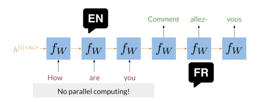
In the image above, you can see a typical RNN that is used to translate the English sentence “How are you?” to its French equivalent, “Comment allez-vous?”. One of the biggest issues with these RNNs, is that they make use of sequential computation. That means, in order for your code to process the word “you”, it has to first go through “How” and “are”. Two other issues with RNNs are the:

• Loss of information: For example, it is harder to keep track of whether the subject is singular or plural as you move further away from the subject.
• Vanishing Gradient: when you back-propagate, the gradients can become really small and as a result, your model will not be learning much.

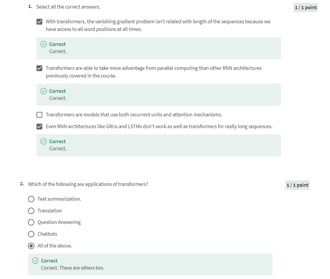
In contrast, transformers are based on attention and don’t require any sequential computation per layer, only a single step is needed. Additionally, the gradient steps that need to be taken from the last output to the first input in a transformer is just one. For RNNs, the number of steps increases with longer sequences. Finally, transformers don’t suffer from vanishing gradients problems that are related to the length of the sequences.

We are going to talk more about how the attention component works with transformers. So don’t worry about it for now 😃

Welcome, this week I’ll teach
you about the transformer model. It’s a purely attention based model
that was developed as Google to remedy some problems with RNNs. First, let me tell you
what these problems are so you understand why
the transformer model is needed. Let’s dive in. First, I will talk about
some problems related to recurrent neural networks using
some familiar architectures. After that, I’ll show you why pure attention
models help us solve those issues. In neural machine translation,
you use a neural architecture to translate from one language to another,
in this example, from English to French. Using an RNN, you have to take
sequential steps to encode your inputs. You start from the beginning
of your input, making computations at every
step until you reach the end. At that point, you decode the information
following a similar sequential procedure. As you can see here, you have to go
through every word in your inputs, starting with the first word, followed
by the second word, one after another. In a sequential matter in order to
start the translation that is done in a sequential way too. For that reason, there is not much
room for parallel computations here. The more words you have
in the input sentence, the more time it will take
to process that sentence. Let’s look closer at a more general
sequence-to-sequence architecture. In this case, to propagate information
from your first word to the last output, you have to go through
capital T sequential steps. Where capital T is an integer that
stands for the number of time steps that your model will go through to process
the inputs of one example sentence. If, for instance, you are inputting
a sentence that consists of five words, then the model will take five times
steps to encode that sentence, and in this example T equals to five.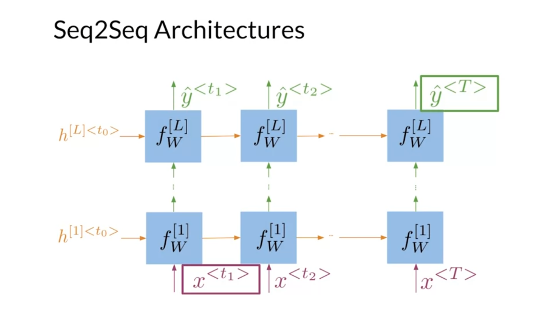

And as you may recall from earlier in
the specialization with large sequences, the information tends to get
lost within the network and. Vanishing gradients problems arise related
to the length of your input sequences. LSTMs and GRUs help a little with these
problems, but even those architectures stop working well when they try to
process very long sequences due to the information bottleneck, as you
saw in the last week of this course. So to recap,
we said we have a loss of information and then we have the vanishing
gradients problem. Including attention in your model
is a way to tackle these problems. You already saw and implemented
a sequence-to-sequence architecture with attention similar to
the one depicted here. Recall that you relied on LSTMs for
your encoder and decoder, but you could also have used GRUs or
just vanilla RNNs. In contrast, transformers rely
only on attention mechanisms and don’t require the use of recurrent
networks in a transformer, attention is all you need. Well, some linear and non-linear
transformations are usually included, but you get the idea.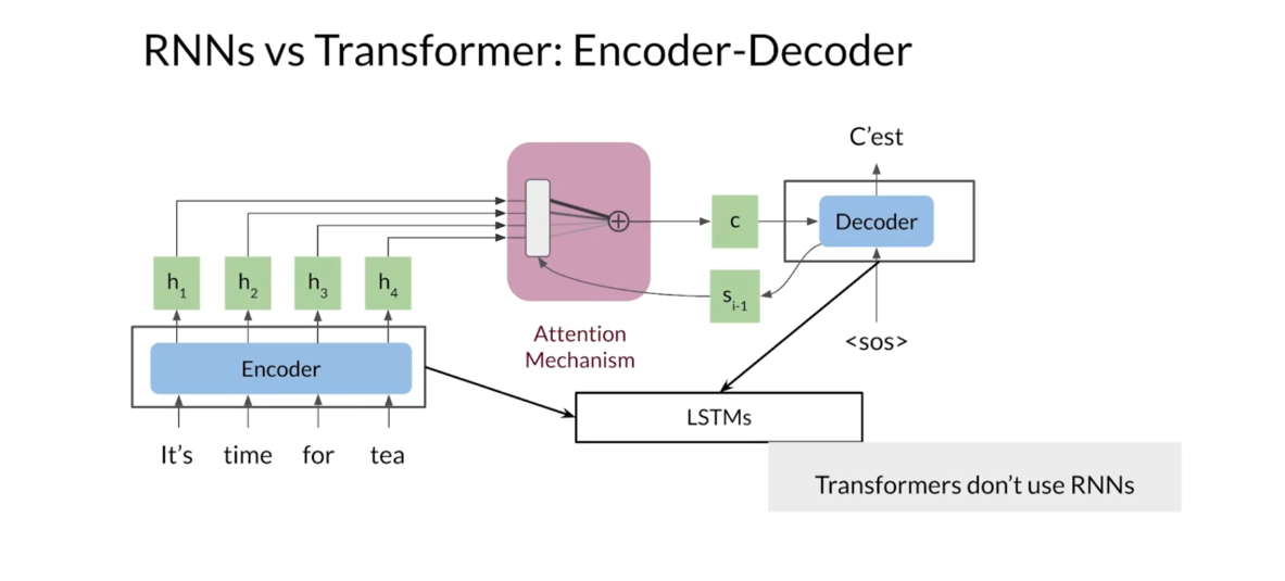

Now you understand why RNNs can be slow
and can have big problems with contexts. These are the cases where
transformers can help. Next, I’ll show you a concrete
overview of the transformers. Let’s go to the next video.

Transformers overview

There has been a lot of
hype with the transformers. In this video, I’ll give you
an overview of the transformers model. The transformer model was introduced
in 2017 by researchers at Google, including Lukasz Kaiser,
who helped us develop this course. Since then, the transformer architecture
has become the standard for large language models, including BERT, T5,
and GPT-3, which you’ll learn about later. The transformers revolutionized the field
of natural language processing. I suggest that you read
the first transformer paper, Attention is all you need. It’s the basis for all the models
presented in the rest of this course. You’ll see how each part of
the transformer model works in detail. But first, I want to give you a brief
overview of this architecture. Now, don’t worry if some of
its components aren’t clear, I’ll go more in depth on
the following lectures. The Transformer model uses
scale dot-product attention, which you saw in the first
week of this course. The first form of attention is very
efficient in terms of computation and memory due to it consisting of just
matrix multiplication operations. This mechanism is
the core of the model and it allows the transformer to grow larger
and more complex while being faster and using less memory than other
comparable model architectures.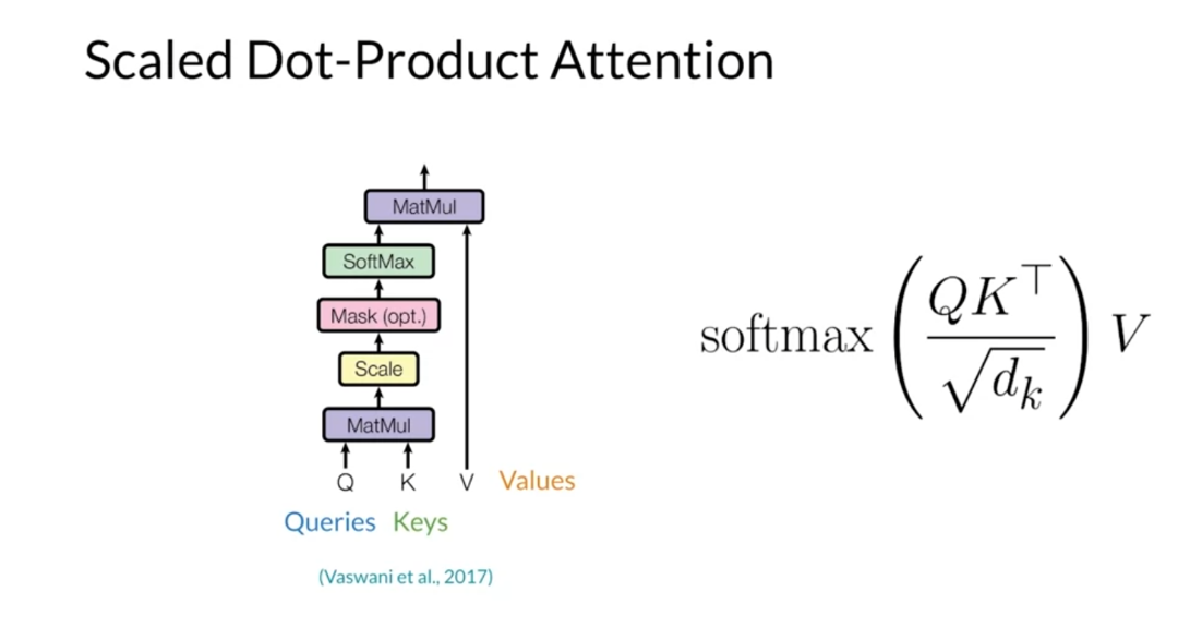

In the transformer model, you will
use the multi-head attention layer. This layer runs in parallel and it has a number of scale dot-product
attention mechanisms and multiple linear transformations of
the input queries, keys, and values. In this layer, the linear transformations
are learnable parameters.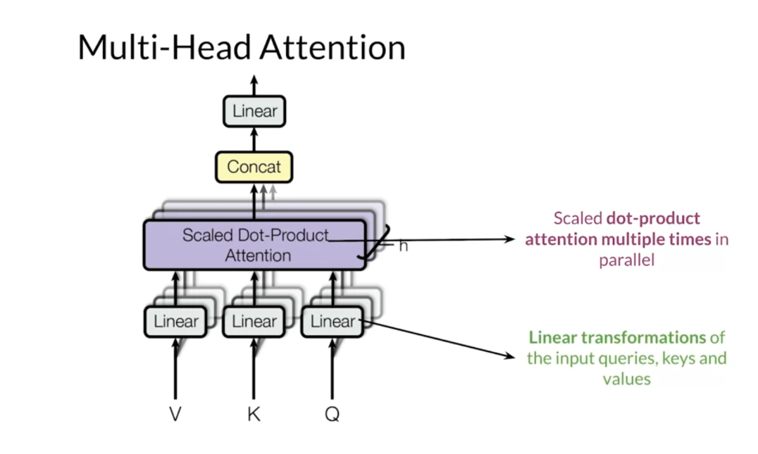

The transformer encoder starts
with a multi-head attention module that performed self attention
on the input sequence. That is, each word in the input attends
to every other word in the input. This is followed by a residual
connection and normalization, a feed forward layer, and another
residual connection and normalization. This entire block is one encoder layer and
is repeated N number of times. Thanks to self attention layer,
the encoder will give you a contextual representation
of each one of your inputs.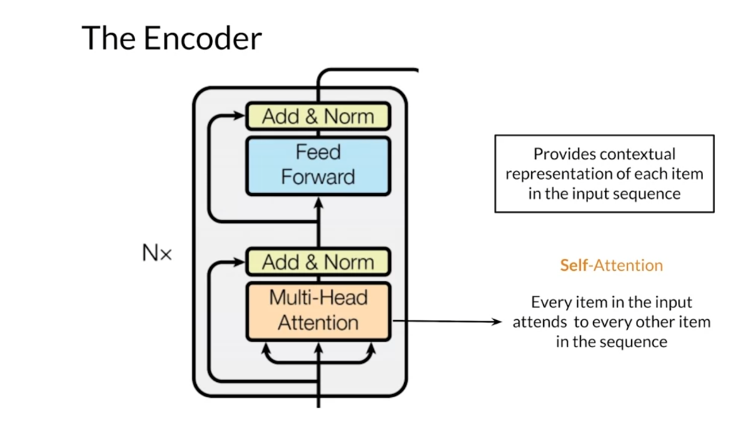

The decoder is constructed similarly
to the encoder with multi-headed attention modules,
residual connections, and normalization. The first attention module is
masked such that each position attends only to previous positions. It blocks leftward flowing information. The second attention module
takes the encoder output and allows the decoder to attend to all items. This whole decoder layer is also repeated
some number of times, one after another.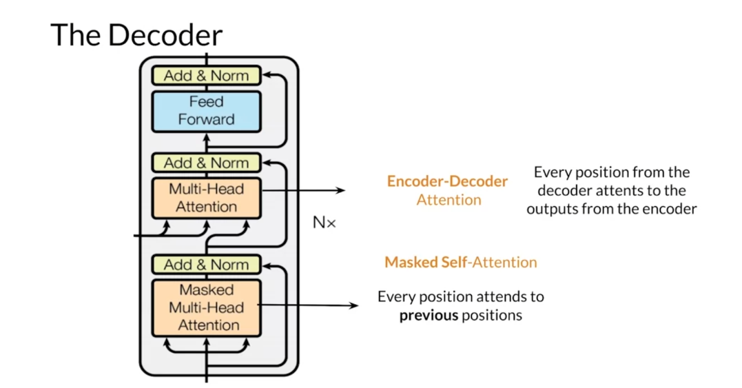

Transformers also incorporates
a positional encoding stage which encodes each input’s position in the sequence. This is necessary because transformers
don’t use recurrent neural networks, but the word order is relevant for
any language. Positional encoding can be learned or
fixed, just as with word embeddings. For instance, let’s suppose you want
to translate from the French phrase. Over here you have [FOREIGN], and then you want to capture
the sequential information. The transformers uses a positional
encoding to retain the position of the input sequence. The positional encoding has values that
are added to the embeddings so that for every input word you have information
about its order and position. In this case, a positional encoding
vector for each word, [FOREIGN].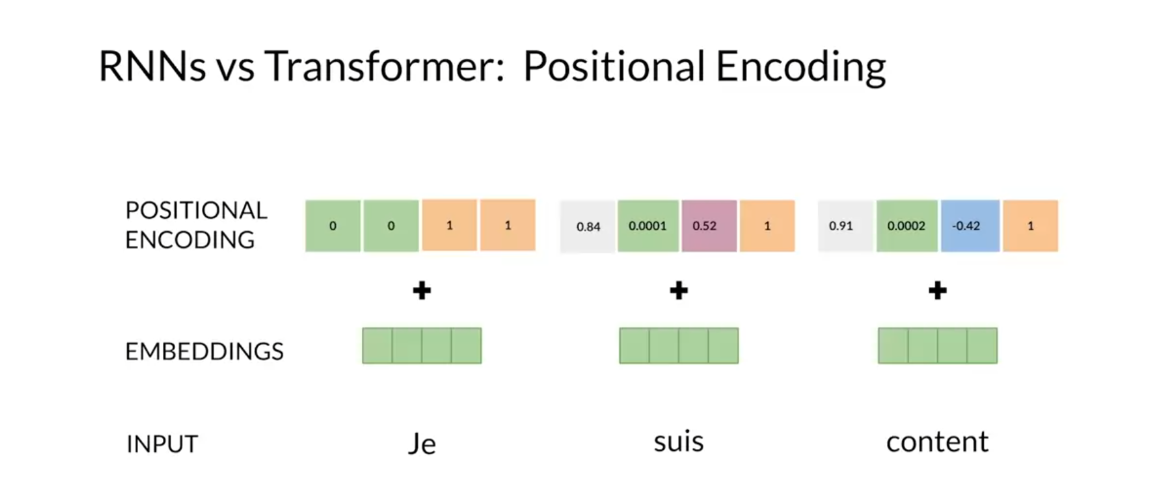

Putting these parts together,
here’s the full model architecture. Briefly on the left,
the input sentence is first embedded and the positional encodings are applied. This goes to the encoder, which consists of multiple layers
of multi-head attention modules. On the right is the decoder,
which takes the output sentence, shifts it over one step to the right,
and the outputs from the encoder. The decoder output is turned
into output probabilities using a linear layer with a softmax activation. This architecture is easy to
parallelize compared to RNN models, and as such, can be trained much more
efficiently on multiple GPUs. It can also scale up to learn multiple
tasks on larger and larger datasets. I went through this quickly but
don’t worry, I’ll go in-depth on each
part in later videos.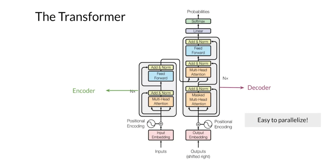

In summary, RNNs have some problems that
come from their sequential structure. With RNNs, it is hard to fully exploit
the advantages of parallel computing. And for long sequences, important
information might get lost within the network and
vanishing gradient problems arise. But fortunately, recent research
has found ways to solve for the shortcomings of RNNs
by using transformers. Transformers are a great alternative
to RNNs that help overcome these problems in NLP and in many fields
that process sequential data. You now can see why everyone
is talking about transformers, they are indeed very useful. In the next video, I’ll talk about some
of the applications of transformers.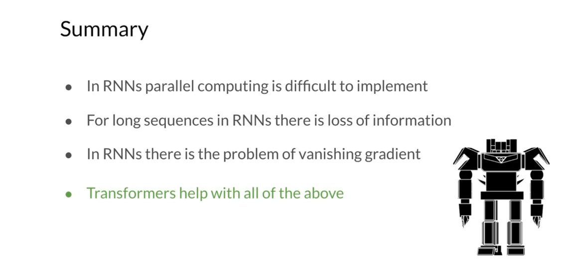

Transformer Applications

Transformer is one of the most
versatile deep learning models. It is successfully applied to a number
of tasks both in NLP and beyond. Let me show you a few examples. >> Speaker 2: In this video you will see a
brief overview of the diverse transformer applications in NLP. Also, you will learn about
some powerful transformers. First, I’ll mention the most popular
applications of transformers in NLP. Then you’ll learn what are the state
of the art transformer models, including the so called text to text
transfer transformer, T5 in shorthand. Finally, you will see how useful and
versatile T5 is. Since transformers can be generally
applied to any sequential task just like RNNs,
it has been widely used throughout NLP. One very interesting and popular application is
automatic text summarization. They’re also used for autocompletion,
named entity recognition, automatic question answering,
machine translation. Another application is chatbots and
many other NLP tasks like sentiment analysis and
market intelligence, among others.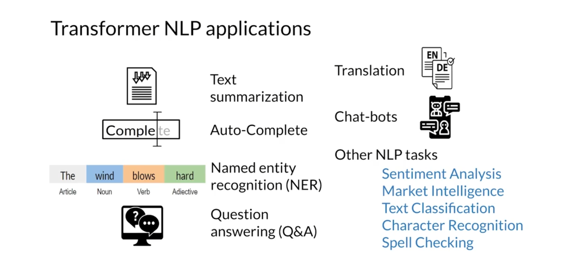

Many variants of transformers
are used in NLP and as usual, researchers give their
models their very own names. For example, GPT-2 which stands for
generative pre-training for transformer, is a transformer
created by OpenAI with pretraining. It is so good at generating text that news
magazines the economists had a reporter ask the GPT-2 model questions as if
they were interviewing a person, and they published the interview
at the end in 2019. Bert, which stands for
bidirectional encoder representations from transformers and which was created
by the Google AI language team, is another famous transformer used for
learning text representations. T5, which stands for
text-to-text transfer transformer and was also created by Google,
is a multitask transformer that can do question answering among
a lot of different tasks.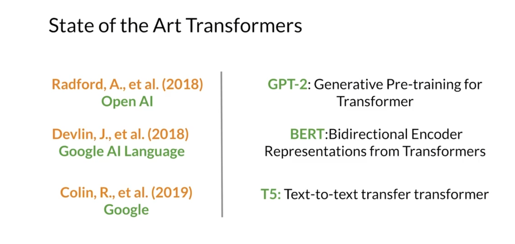

Let’s dive a little bit
deeper into the T5 model. A single T5 model can learn to
do multiple different tasks. This is pretty significant advancement. For example, let’s say you want to
perform tasks such as translation, classification, and question answering. Normally, you would design and train
one model to perform translation, and then design and train a second model
to perform classification, and then design and train a third model
to perform question answering. But with transformers, you can train a single model that is
able to perform all of these tasks. For instance, to tell the T5 model that
you wanted to perform a certain task, you’ll give the model an input string of
text that includes both the task that you want it to do, as well as the data
that you want it to perform that task on. For example, if you want to translate
the particular English sentence, I am happy from English to French, you would use the input string translates
English into French colon I am happy. And the model would be able to
output the sentence [FOREIGN], which is the translation
of I’m happy in French. This is an example of classification over
here, where input sentences are classified into two classes, acceptable when
they make sense and unacceptable. In this example, the input string
starts with cola sentence, which the model understands
is asking it to classify the sentence that follows this
command as acceptable or unacceptable. For instance, the sentence he
bought fruits and is incomplete and then is classified as unacceptable. Meanwhile, if we give the T5
model this input cola sentence, he bought fruits and vegetables. The model classifies he bought fruits and
vegetables as an acceptable sentence. If we give the T5 model the input starting
with the word question over here, followed by a colon, the model then knows
that this is a question answering example. In this example, the question is which volcano in Tanzania
is the highest mountain in Africa? And your T5 will output the answer to that
question, which is Mount Kilimanjaro. And remember that all of these tasks
are done by the same model with no modification other than the input
sentences, how cool is that?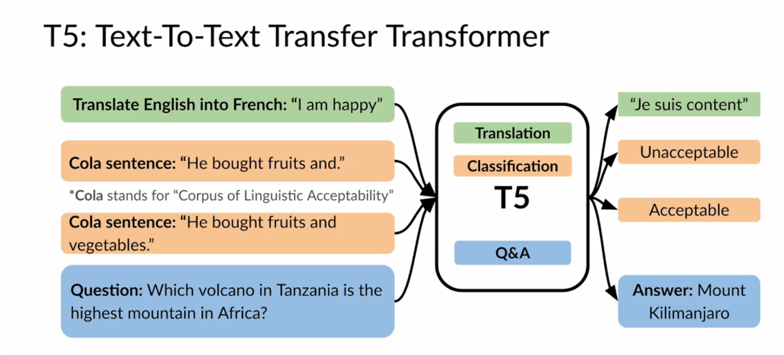

Even more, the T5 also performs tasks
of regression and summarization. Recall that a regression model is one
that outputs a continuous numeric value. Here you can see an example of regression
which outputs the similarity between two sentences. The start of the input string Stsb
will indicate to the model that it should perform a similarity
measurement between two sentences. The two sentences are denoted by
the words sentence1 and sentence2. The range of possible outputs for this
model is any numerical value ranging from zero to five, where zero indicates that
the sentences are not similar at all and five indicates that
the sentences are very similar. Let’s consider this example when
comparing the sentence 1, cats and dogs are mammals with sentence 2,
these are four known forces in nature, gravity, electromagnetic,
weak, and strong. The resulting similarity level is zero, indicating that the sentences
are not similar. Now let’s consider this other example. Sentence1, cats and dogs are mammals. And sentence 2, cats, and dogs,
and cows are domesticated. In this case, the similarity level may be 2.6 if you
use a range between zero and five. Finally, here you can see
an example of summarization. It is a long story about all
the events and details of an onslaught of severe weather in Mississippi,
which is summarized just as six people hospitalized after
a storm in Attala county.

This is a demo using T5 for
trivia questions so that you can compete
against a transformer. What makes this demo interesting is
that T5 was trained in a closed book setting without access to
any external knowledge. So these are examples where I
was playing against the trivia. All right, so in this video you saw what
are the transformers applications in NLP, which range from translations
to summarization. Some transformers include GPT,
BERT and T5. And I also showed you how versatile and
powerful T5 is, as it can perform multiple tasks
using tech representations.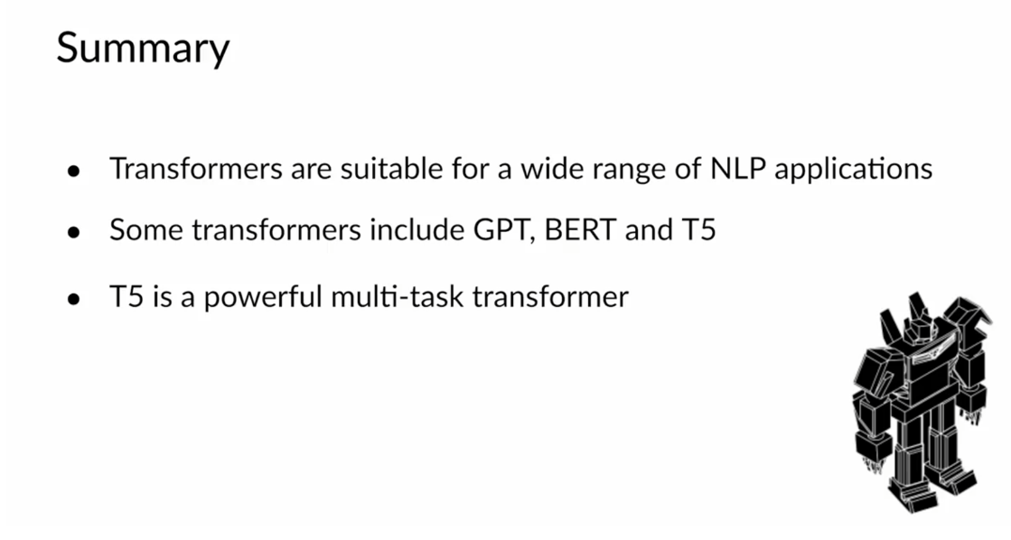

Now you know why we need
transformers and where it can be applied. Isn’t it astounding this one model
can handle such a variety of tasks? I hope you are now eager to
learn how transformers works. And that’s what I will show you next. Let’s go to the next video.

Scaled and Dot-Product Attention

The main operation and transformer
is the scale dot product attention. You’ve already seen attention in
the first week of this course. In this video,
I’ll remind you how it works. First, I’ll remind you of the formula
used for scale dot products attention. Then you’ll see some
details about the math and the dimensions of the queries keys and
values. Recall that in scaled dot-products
attention, you have queries, keys and values. The attention layer outputs
contacts vectors for each query. And the context vectors are weighted
sums of the values where the similarity between the queries and keys determines
the weights assigned to each value. The SoftMax ensures that the weights add
up to 1 and the division by the square roots of the dimension of the key
factors is used to improve performance. The scale dot-product attention
mechanism is very efficient since it relies only on matrix multiplication and
SoftMax. Additionally, you could implement this
attention mechanism to run on GPUs or TPUs to speed up training.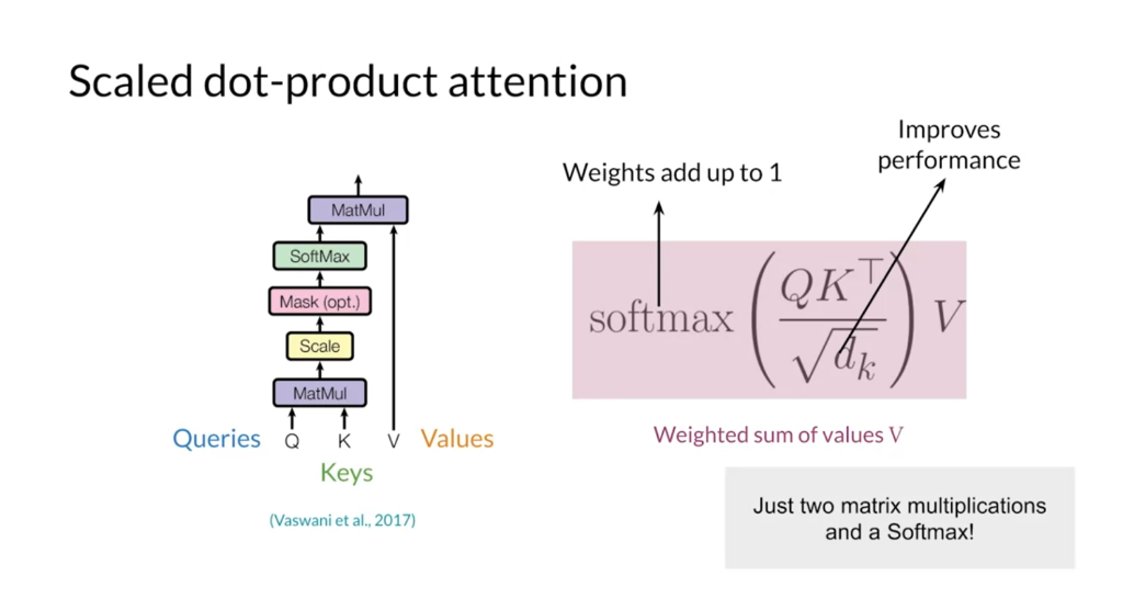

To get the query, key and value matrices,
you must first transform the words in your sequences toward embedding’s,
let’s take the sentence. Je suis heureux are source for
the queries. You’ll need to get the embedding
vector for the word Je. Then for the words suis and
finally for the word heureux. The query matrix will contain all
of these embedding vectors as rows. Not that the matrix sizes given by
the size of the word embeddings and the length of the sequence. To get the key matrix let’s use
a source of the sentence I am happy. You will get the embedding for
each word in the sentence and stack them together to
form the key matrix. You will generally use the same
vectors used for the key matrix for the value matrix. But you could also transform them first. Note however, that the number of
vectors used to form the key and value matrix must be the same.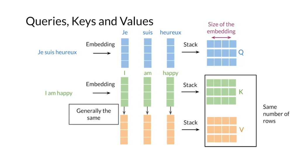

Now you can revisit the scale attention
formula that I showed you before to get a sense of the dimensions of
the matrices involved at every time step. First, you compute the matrix
products between the query and the transpose of the key matrix. You scale it by the inverse of the square
of the dimension of the key vectors, D sub K and calculate the SoftMax. This competition will give you a matrix
with the weights for each keeper query. Therefore the weight matrix
will have a total number of elements equal to the number of
queries times the number of keys. And thus matrix, the third element in
the second row would correspond to the weights assigned to the third key for
the second query. After the computation
of the weights matrix, you can multiply it with the value
matrix to get a matrix that has rows and the context vector
corresponding to each query. And the number of columns on this matrix
is equal to the size of the value vectors, which is often the same
as the embedding size.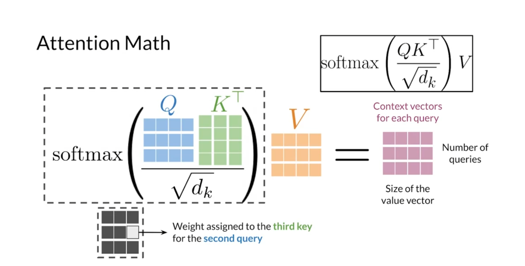

Scale dot-product attention is
the heart and soul of transformers. In general terms,
this mechanism takes queries, keys and values as matrices of embedding’s. It is composed of just two matrix
multiplication and a SoftMax function. Therefore, you could
consider using GPUs and TPUs to speed up the training of
models that rely on this mechanism. Now you understand that
products attention very well. In the transformer decoder, we need an extended version
called the self-masked attention. I’ll teach you about it in the next video.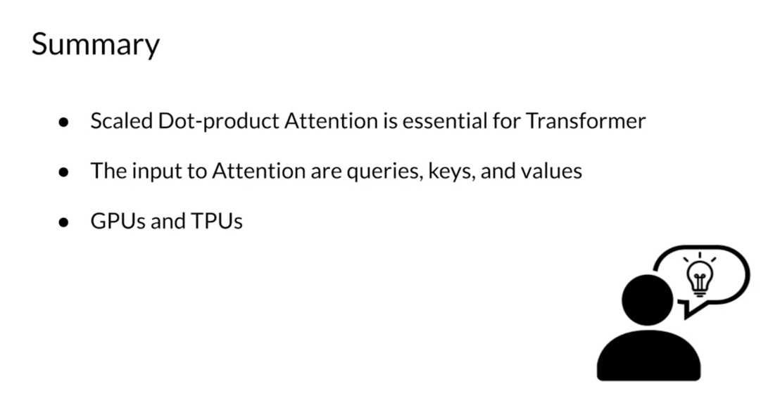

在注意力机制（Attention Mechanism）中，除以根号下 dk 的作用是对注意力权重进行缩放（scale）。这个缩放是为了使得注意力权重的分布更加稳定和平滑，有助于减少训练中的梯度消失或梯度爆炸问题。

在注意力机制中，计算注意力权重的一般公式为：

$$\text{Attention}(Q,K,V)=\text{softmax}\left(\frac{Q{K}^T}{\sqrt{d_k}}\right)V$$
其中，(Q)、(K) 和 (V) 分别代表查询（Query）、键（Key）和值（Value）的矩阵表示。($d_k$) 是键的维度（dimension of key），也就是每个键的长度。在计算注意力权重时，将查询和键的点积除以 ($\sqrt{d_k}$) 进行缩放，最后使用 softmax 函数将缩放后的值转换为注意力权重。

缩放的主要目的是控制点积的值域，使得在计算 softmax 时更加稳定，避免出现很大的数值，从而提高模型的训练效果。

在注意力机制中，通常将注意力机制的输入表示为三个矩阵：查询矩阵 Q、键矩阵 K 和值矩阵 V。这些矩阵的行数通常表示输入序列的长度，列数则表示特征向量的维度。

在计算注意力权重时，Q 和 K 矩阵进行点积操作，得到的矩阵再除以 $\sqrt{d_k}$ 进行缩放。这里的 $d_k$ 通常指的是矩阵 K 的列数，也就是键矩阵中每个键的长度。这个操作的目的是使得点积的结果更加稳定，有助于控制梯度的大小。

Masked Self Attention

In this video, I’ll review the different types of attention mechanisms in
the transformer model, and you will see how to
compute masked self-attention. First, you will see what the three main ways of attention in the
transformer model are. Afterwards, I’ll show you a brief overview of
masked self-attention. One of the attention
mechanisms in a transformer model is the familiar
encoder-decoder attention. In that mechanism, the words in one sentence attend to all other words
in another one. That is, the queries come from one sentence while the keys
and values come from another. You’ve already used this
kind of attention in the translation task
from last week, where the words from
sentences in French attended towards from
sentences in English.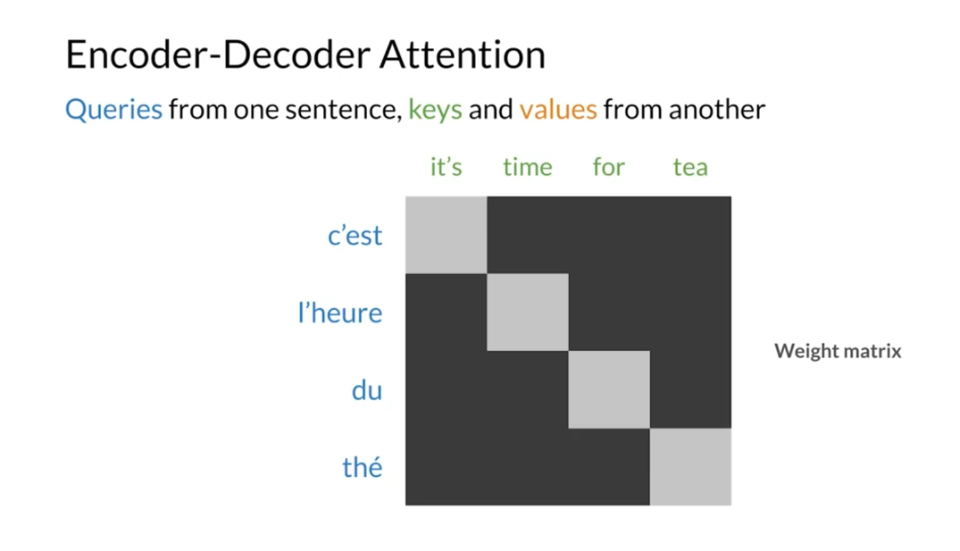

Self-attention, the queries, keys, and values come
from the same sentence. Every word attends to every
other word in the sequence. This type of attention
lets you get contextual representations
of your words. In other terms,
self-attention gives you a representation of the meaning of each word within
the sentence.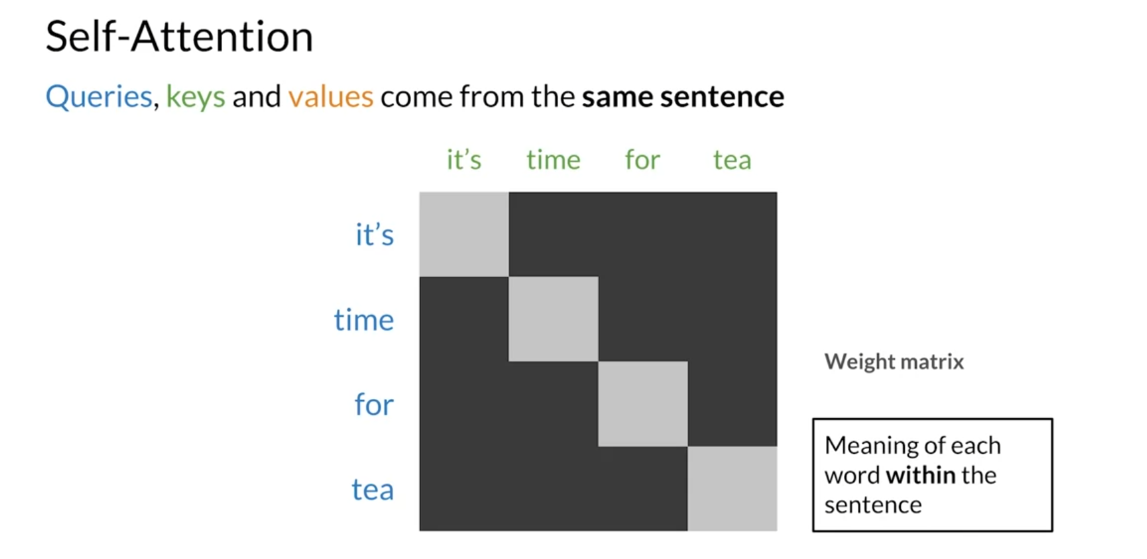

Finally, in masked
self-attention queries, keys and values also come
from the same sentence, but each query cannot attend
to keys on future positions. This attention
mechanism is present in the decoder from
the transformer model and ensures that predictions at each position depend only
on the known outputs.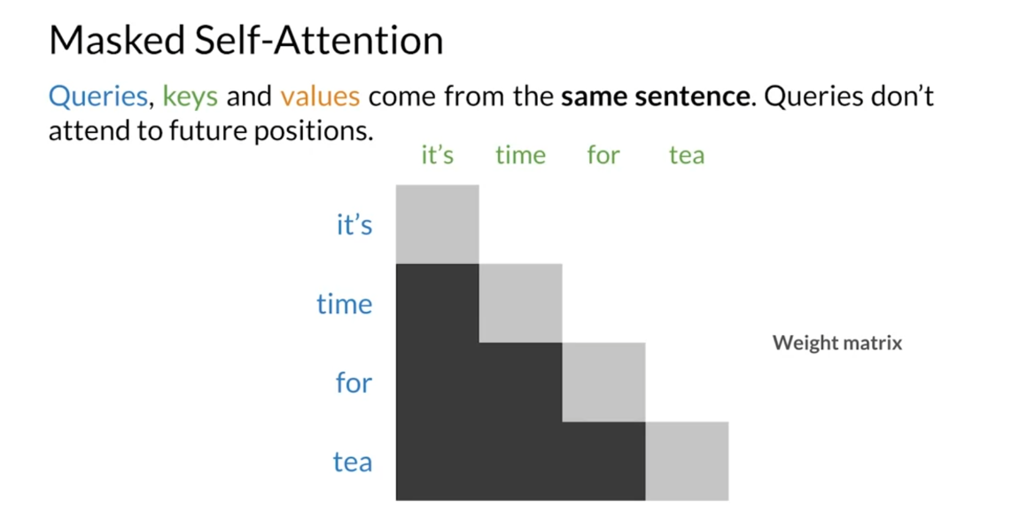

Mathematically,
self-attention works precisely as the
encoder-decoder attention. The only difference
is the nature of the inputs for each mechanism. Let’s focus on masked
self-attention. Recall that the scale
dot-product attention requires the calculation of the softmax of the
scaled products between the queries and the
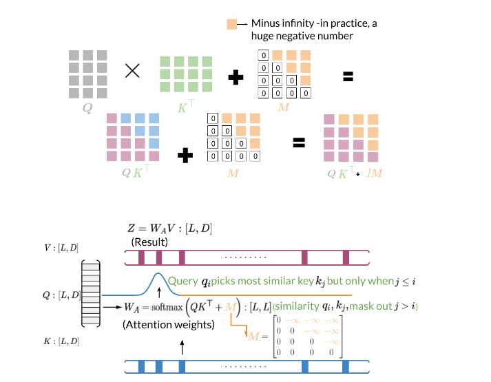
transpose of the key matrix. Then for mask self-attention, you add a mask matrix
within the softmax. The mask has a zero on
all of its positions, except for the elements
above the diagonal, which are set to minus infinity. Or in practice, a
huge negative number. After taking the softmax, this addition ensures
that the elements in the weights matrix are zero for all the keys and the subsequent
positions to the query. In the end, as with the
other types of attention, you multiply the weights
matrix by the value matrix to get the context vector for
each query, and that’s it. You only need to
add a matrix within the softmax to ensure that the queries don’t
attend to future positions.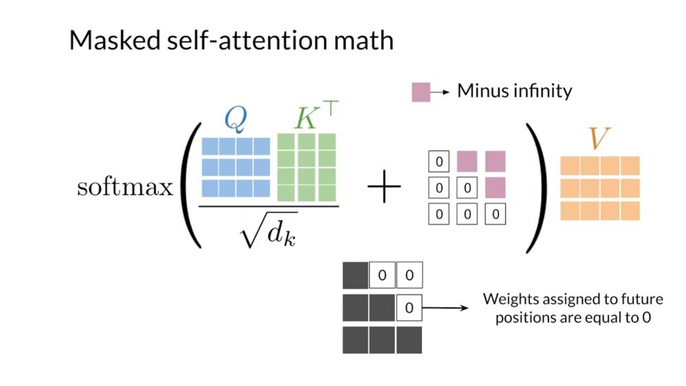

当输入中包含负无穷时，Softmax 函数会使得对应的输出值接近于零。具体来说，如果输入向量中存在一个或多个元素为负无穷（即 ($-\infty$）)，那么对应的 Softmax 输出值将会是零。

例如，考虑一个包含负无穷的输入向量 ([-1,$ -\infty$, -3])，经过 Softmax 函数计算后，我们得到：

$$\text{softmax}([-1,-\infty ,-3])=\left[\frac{e^{-1}}{e^{-1}+e^{-\infty }+e^{-3}},\frac{e^{-\infty }}{e^{-1}+e^{-\infty }+e^{-3}},\frac{e^{-3}}{e^{-1}+e^{-\infty }+e^{-3}}\right]$$
由于 ($e^{-\infty }$) 在数值上表示一个极小的值，可以近似为零，因此上述计算可以简化为：

$$\text{softmax}([-1,-\infty ,-3])=[0.8808,0,0.1192]$$
其中第二个元素的值接近于零。这表明，当输入中存在负无穷时，Softmax 函数会使得对应的输出值趋近于零。

In this video, I showed you the three main
ways of attention. Encoder-decoder attention, self-attention, and
masked self-attention. In masked self-attention, queries and keys are contained
in the same sentence, but queries can not attend
to future positions. You have seen many types
of attention so far. In the next video, I’ll show you the
multi-headed attention. It is a very powerful form of attention that allows
for parallel computing.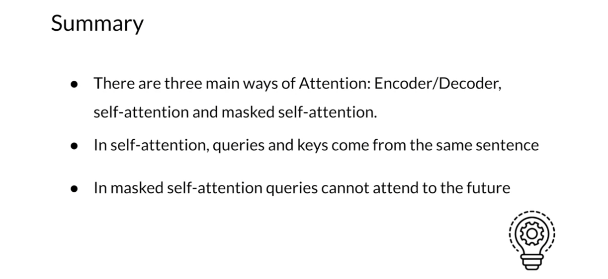

假设我们使用了一个简单的自注意力机制来处理句子 “我 喜欢 你”。在这个机制中，我们计算了每个位置对其他位置的注意力权重，最终得到了一个注意力权重矩阵。这个矩阵的含义是，在生成每个词语时，模型应该给予句子中其他位置的词语多少注意力。

以句子 “我 喜欢 你” 为例，假设我们使用上面的方法计算了注意力权重矩阵：

Attention Weights = [ 0.7 0 0 0.2 0.6 0 0.1 0.3 0.6 ] \text{Attention Weights} = [0.7000.20.600.10.30.6]

Attention Weights= ​0.70.20.1​00.60.3​000.6​ ​
其中每一行代表句子中一个词语的注意力权重，例如第一行表示生成 “我” 这个词时，对 “我” 这个位置的词语（即 “我” 自身）的注意力权重为 0.7，对 “喜欢” 和 “你” 的注意力权重为 0。

这个注意力权重矩阵告诉了模型在生成每个词语时应该关注句子中的哪些位置，这有助于模型更好地理解句子的语义和结构。

假设我们有一个注意力分数矩阵 (A)，形状为 ($3\times 3$)，表示一个句子中每个词对其他词的注意力权重。同时，我们有一个值矩阵 (V)，形状也为 ($3\times 3$)，表示每个词的值向量。那么将注意力分数矩阵与值矩阵相乘的结果 ($A\times V$) 的含义如下：

1. 矩阵形状：乘积的形状仍为 ($3\times 3$)，因为每个注意力分数与对应的值向量相乘得到一个新的值向量。

2. 含义：结果矩阵中的每个元素表示该位置上词语的加权值向量。换句话说，它表示每个词语根据其他词语的注意力权重加权后的值向量。

3. 每一行代表：每一行表示一个词语根据其他所有词语的注意力权重加权后的值向量。这可以理解为每个词语在不同注意力下的表示。

4. 每一列代表：每一列表示一个词语的值向量在不同位置上经过注意力权重加权后的结果。这可以理解为每个词语对整个句子的注意力分布。

总之，($A\times V$) 的结果表示了句子中每个词语根据其他词语的注意力权重加权后的值向量，是注意力机制的核心操作之一，有助于模型更好地理解输入句子的语义和结构。

在矩阵乘法 ($A\times V$) 中，每一行代表了输入序列中的一个词在经过注意力加权后的值向量，这个值向量可以理解为该词在上下文中的重要性或者对应的语义信息。因此，在这个矩阵中，每一行是重要的，而不是每一列。

Multi-head Attention

You have learned all the basics
of attention by now. In fact, you could already
build a transformer from it. But if you want it to work really well,
run fast and get very good results, you’ll need one more thing. The multi-head attention. Let me show you what it is. First, I’ll share with you some
intuition on multi-head attention. Afterwards, I’ll show
you the math behind it. Recall that you need word embeddings for
the query key and value matrices in scaled
dot-product attention. In multi-head attention, you apply in parallel the attention
mechanism to multiple sets of these matrices that you can get by
transforming the original embeddings. In multi-head attention, the number
of times that you apply the attention mechanism is the number
of heads in the model. For instance, you will need
two sets of queries, keys and values in a model with two heads. The first head would use
a set of representations and the second head would use a different set. In the transformer model,
you’d get different representations by linearly transforming the original
embeddings by using a set of matrices W superscripts QKV for
each head in the model. Using different sets of representations,
allow your model to learn multiple relationships between the words
from the query and key matrices.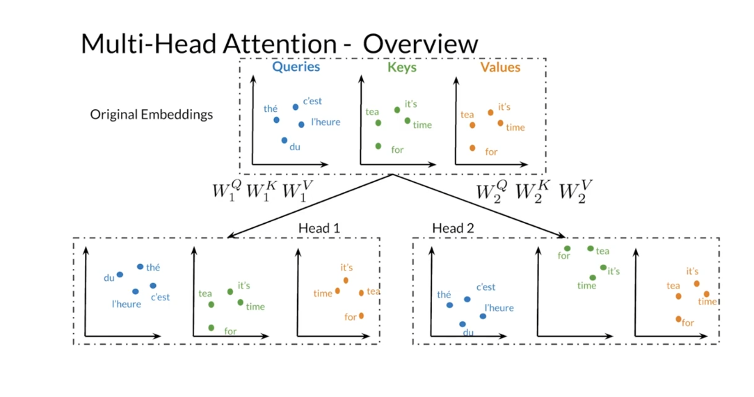

With that in mind, let me show you
how multi-head attention works. The inputs to multi-head detention
is the value key and query matrices. First, you transform each of these
matrices into multiple vector spaces. As you saw previously,
the number of transformations for each matrix is equal to
the number of heads in the model. Then you will apply the scaled
dot-product attention mechanism to every set of value, key and
query transformations, where again the number of sets is equal
to the number of heads in the model. After that, you concatenate
the results from each head in the model into a single matrix. Finally, you transform the resulting
matrix to get the output context vectors. Note that every linear transformation
in multi-head attention contains a set of learnable parameters, so let’s go
through every step in more detail.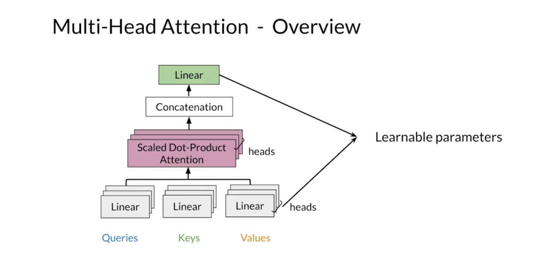

Say that you have two heads in your model. The inputs to the multi-head attention
layer are the queries, keys, and values matrices. The number of columns in those
matrices is equal to d sub model, which is the embedding size, and
the number of rows is given by the number of words the sequences used
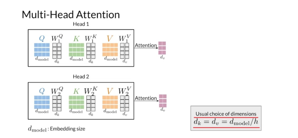
to construct each matrix. The first step is to transform the
queries, keys and values using a set of matrices W superscripts, QK and
V per head of the model. This step will give you the different
sets of representations that you use for the parallel attention mechanisms. The number of rows and the transformation
matrices is equal to d sub model. The number of columns d sub K for
the queries and keys transformation matrices, and
the number of columns d sub V for W superscript V are hyperparameters
that you can choose. |n the original transformer model, the author advises setting d sub K and
d sub V equals to the dimension of the embeddings divided
by the number of heads in the model. This choice of sizes would ensure that
the computational cost of multi head attention doesn’t exceed by much
the one for a single head attention. After getting the transformed values for
the query key and value matrices per head, you can apply in parallel
the attention mechanism. As a result, you get a matrix per head
with the column dimensions equal to d sub V, and the number of rows in those
matrices is the same as the number of rows in the query matrix. Then you concatenate horizontally
the matrices outputted by each attention head in the model. So you will get a matrix that has d sub
V times the number of heads columns. Then you apply a linear transformation W
superscript O to the concatenated matrix. This linear transformation has
columns equal to d sub model, and if you choose d sub V to be equal to
the embedding size divided by the number of heads, the number of rows in this
matrix would also be d sub model. Just as with single head attention,
you will get a matrix with the context vectors of size d sub model for
each of your original queries. That’s it for multi-head attention, you
just need to apply the attention mechanism to multiple sets of representations for
the queries, keys, and values. Then you concatenate the results from each
attention computation to get a matrix that you linearly transform to get the
context vectors for each original query.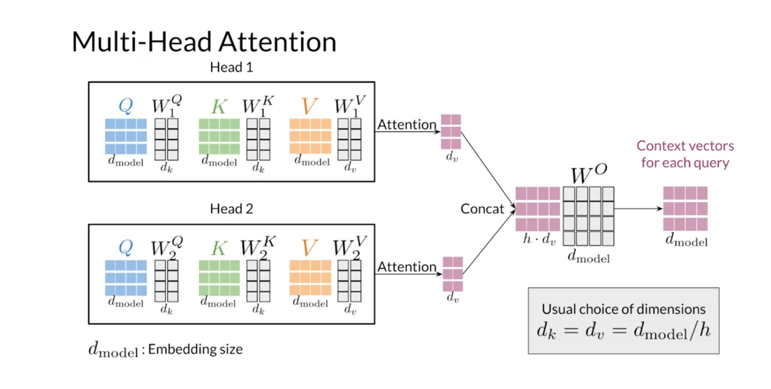

In this video, you learned how
multi-head attention works and you saw some of the dimensions of the parameter
matrices involved in its calculations. You can implement multi-head attention
to make computations in parallel. And with a proper choice of sizes for
the transformation matrices, the total computational time is similar
to the one of single head attention. In the last three videos,
you learned about attention. You know the basic dot product attention,
the causal one, and the multi-headed one. You’re now ready to build
your own transformer decoder. That’s what we’ll do in the next video.

Reading: Multi-head Attention

In this reading, you will see a summary of the intuition behind multi-head attention and scaled dot product attention.

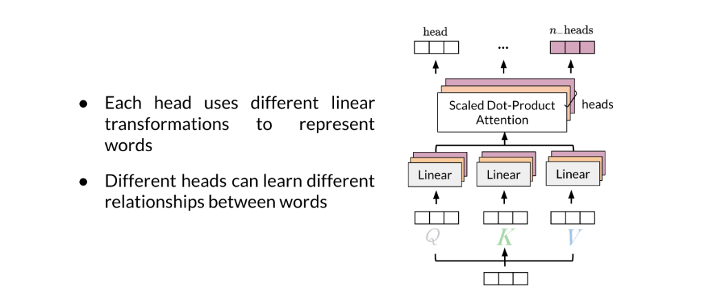
Given a word, you take its embedding then you multiply it by the $W_Q,W_K,W_V$ matrix to get the corresponding queries, keys and values. When you use multi-head attention, each head performs the same operation, but using its own matrices and can learn different relationships between words than another head.

Here is step by step guide, first you get the Q, K, V matrices:

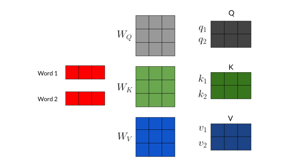
For each word, you multiply it by the corresponding $W_Q,W_K,W_V$ matrices to get the corresponding word embedding. Then you have to calculate scores with those embedding as follows:

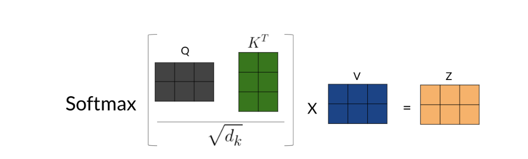
Note that the computation above was done for one head. If you have several heads, concretely $n$, then you will have $Z_1,Z_2,...,Z_n$.In which case, you can just concatenate them and multiply by a $W_O$ matrix as follows:

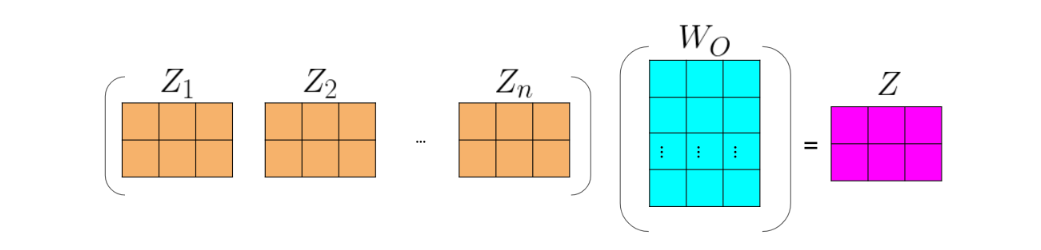
In most cases, the dimensionality of Zs is configured to align with the $d_{model}$ (given that the head size is determined by $d_{head}=d_{model}/h)$, ensuring consistency with the input dimensions. Consequently, the combined representations (embeddings) typically undergo a final projection by $W_o$ into an attention embedding without changes in dimensions.

Forinstance, if $d_{model}$ is 16, with two heads, concatenating $Z_1$and $Z_2$ results in a dimension of 16(8+8). Similarly, with four heads, the concatenation of $Z_1,Z_2,Z_3$ and $Z_4$ also results in a dimension of 16(4+4+4+4). In this example, and in most common architectures, it’s noteworthy that the number of heads does not alter the dimensionality of the concatenated output. This holds true even after the final projection with $W_o$, which, too, typically maintains consistent dimensions.

Lab: Attention

The Three Ways of Attention and Dot Product Attention: Ungraded Lab Notebook

In this notebook you’ll explore the three ways of attention (encoder-decoder attention, causal attention, and bi-directional self attention) and how to implement the latter two with dot product attention.

Background

As you learned last week, attention models constitute powerful tools in the NLP practitioner’s toolkit. Like LSTMs, they learn which words are most important to phrases, sentences, paragraphs, and so on. Moreover, they mitigate the vanishing gradient problem even better than LSTMs. You’ve already seen how to combine attention with LSTMs to build encoder-decoder models for applications such as machine translation.

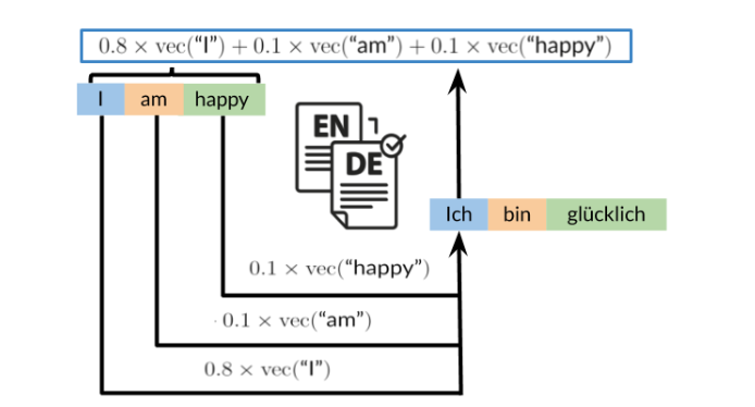
This week, you’ll see how to integrate attention into transformers. Because transformers do not process one token at a time, they are much easier to parallelize and accelerate. Beyond text summarization, applications of transformers include:

• Machine translation
• Auto-completion
• Named Entity Recognition
• Chatbots
• Question-Answering
• And more!

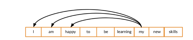
Along with embedding, positional encoding, dense layers, and residual connections, attention is a crucial component of transformers. At the heart of any attention scheme used in a transformer is dot product attention, of which the figures below display a simplified picture:

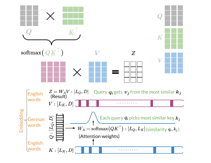
With basic dot product attention, you capture the interactions between every word (embedding) in your query and every word in your key. If the queries and keys belong to the same sentences, this constitutes bi-directional self-attention. In some situations, however, it’s more appropriate to consider only words which have come before the current one. Such cases, particularly when the queries and keys come from the same sentences, fall into the category of causal attention.

For causal attention, you add a mask to the argument of our softmax function, as illustrated below:

Now let’s see how to implement the attention mechanism.

Imports

import os
os.environ['TF_CPP_MIN_LOG_LEVEL'] = '3'

import sys

import tensorflow as tf

import textwrap
wrapper = textwrap.TextWrapper(width=70)

1
2
3
4
5
6
7
8
9
10

Here is a helper function that will help you display useful information:

• display_tensor() prints out the shape and the actual tensor.

def display_tensor(t, name):
    """Display shape and tensor"""
    print(f'{name} shape: {t.shape}\n')
    print(f'{t}\n')
1
2
3
4

Create some tensors and display their shapes. Feel free to experiment with your own tensors. Keep in mind, though, that the query, key, and value arrays must all have the same embedding dimensions (number of columns), and the mask array must have the same shape as tf.matmul(query, key_transposed).

q = tf.constant([[1.0, 0.0, 0.0], [0.0, 1.0, 0.0]])
display_tensor(q, 'query')
k = tf.constant([[1.0, 2.0, 3.0], [4.0, 5.0, 6.0]])
display_tensor(k, 'key')
v = tf.constant([[0.0, 1.0, 0.0], [1.0, 0.0, 1.0]])
display_tensor(v, 'value')
m = tf.constant([[1.0, 0.0], [1.0, 1.0]])
display_tensor(m, 'mask')
1
2
3
4
5
6
7
8

Output

query shape: (2, 3)

[[1. 0. 0.]
 [0. 1. 0.]]

key shape: (2, 3)

[[1. 2. 3.]
 [4. 5. 6.]]

value shape: (2, 3)

[[0. 1. 0.]
 [1. 0. 1.]]

mask shape: (2, 2)

[[1. 0.]
 [1. 1.]]
1
2
3
4
5
6
7
8
9
10
11
12
13
14
15
16
17
18
19

Dot product attention

Here you compute
$\text{softmax}\left(\frac{Q{K}^T}{\sqrt{d}}+M\right)V$, where the (optional, but default) scaling factor $\sqrt{d}$ is the square root of the embedding dimension.

penultimate: 倒数第二个

def dot_product_attention(q, k, v, mask, scale=True):
    """
    Calculate the attention weights.
      q, k, v must have matching leading dimensions.
      k, v must have matching penultimate dimension, i.e.: seq_len_k = seq_len_v.
      The mask has different shapes depending on its type(padding or look ahead) 
      but it must be broadcastable for addition.

    Arguments:
        q (tf.Tensor): query of shape (..., seq_len_q, depth)
        k (tf.Tensor): key of shape (..., seq_len_k, depth)
        v (tf.Tensor): value of shape (..., seq_len_v, depth_v)
        mask (tf.Tensor): mask with shape broadcastable 
              to (..., seq_len_q, seq_len_k). Defaults to None.
        scale (boolean): if True, the result is a scaled dot-product attention. Defaults to True.

    Returns:
        attention_output (tf.Tensor): the result of the attention function
    """
    
    # Multiply q and k transposed.
    matmul_qk = tf.matmul(q, k, transpose_b=True)  # (..., seq_len_q, seq_len_k)

    # scale matmul_qk with the square root of dk
    if scale:
        dk = tf.cast(tf.shape(k)[-1], tf.float32)
        matmul_qk = matmul_qk / tf.math.sqrt(dk)
    # add the mask to the scaled tensor.
    if mask is not None:
        matmul_qk = matmul_qk + (1. - mask) * -1e9 

    # softmax is normalized on the last axis (seq_len_k) so that the scores add up to 1.
    attention_weights = tf.keras.activations.softmax(matmul_qk)

    # Multiply the attention weights by v
    attention_output = tf.matmul(attention_weights, v)  # (..., seq_len_q, depth_v)

    return attention_output
1
2
3
4
5
6
7
8
9
10
11
12
13
14
15
16
17
18
19
20
21
22
23
24
25
26
27
28
29
30
31
32
33
34
35
36
37
38

Finally, you implement the masked dot product self-attention (at the heart of causal attention) as a special case of dot product attention

def causal_dot_product_attention(q, k, v, scale=True):
    """ Masked dot product self attention.
    Args:
        q (numpy.ndarray): queries.
        k (numpy.ndarray): keys.
        v (numpy.ndarray): values.
    Returns:
        numpy.ndarray: masked dot product self attention tensor.
    """
    
    # Size of the penultimate dimension of the query
    mask_size = q.shape[-2]

    # Creates a matrix with ones below the diagonal and 0s above. It should have shape (1, mask_size, mask_size)
    mask = tf.experimental.numpy.tril(tf.ones((mask_size, mask_size)))  
    
    return dot_product_attention(q, k, v, mask, scale=scale)
1
2
3
4
5
6
7
8
9
10
11
12
13
14
15
16
17

result = causal_dot_product_attention(q, k, v)
display_tensor(result, 'result')
1
2

Output

result shape: (2, 3)

[[0.         1.         0.        ]
 [0.8496746  0.15032543 0.8496746 ]]
1
2
3
4

Lab: Masking

In this lab, you will implement the masking, that is one of the essential building blocks of the transformer. You will see how to define the masks and test how they work. You will use the masks later in the programming assignment.

import os
os.environ['TF_CPP_MIN_LOG_LEVEL'] = '3'
import tensorflow as tf
1
2
3

1 - Masking

There are two types of masks that are useful when building your Transformer network: the padding mask and the look-ahead mask. Both help the softmax computation give the appropriate weights to the words in your input sentence.

1.1 - Padding Mask

Oftentimes your input sequence will exceed the maximum length of a sequence your network can process. Let’s say the maximum length of your model is five, it is fed the following sequences:

[["Do", "you", "know", "when", "Jane", "is", "going", "to", "visit", "Africa"], 
 ["Jane", "visits", "Africa", "in", "September" ],
 ["Exciting", "!"]
]
1
2
3
4

which might get vectorized as:

[[ 71, 121, 4, 56, 99, 2344, 345, 1284, 15],
 [ 56, 1285, 15, 181, 545],
 [ 87, 600]
]
1
2
3
4

When passing sequences into a transformer model, it is important that they are of uniform length. You can achieve this by padding the sequence with zeros, and truncating sentences that exceed the maximum length of your model:

[[ 71, 121, 4, 56, 99],
 [ 2344, 345, 1284, 15, 0],
 [ 56, 1285, 15, 181, 545],
 [ 87, 600, 0, 0, 0],
]
1
2
3
4
5

Sequences longer than the maximum length of five will be truncated, and zeros will be added to the truncated sequence to achieve uniform length. Similarly, for sequences shorter than the maximum length, zeros will also be added for padding.

When pasing these vectors through the attention layers, the zeros will typically disappear (you will get completely new vectors given the mathematical operations that happen in the attention block). However, you still want the network to attend only to the first few numbers in that vector (given by the sentence length) and this is when a padding mask comes in handy. You will need to define a boolean mask that specifies to which elements you must attend (1) and which elements you must ignore (0) and you do this by looking at all the zeros in the sequence. Then you use the mask to set the values of the vectors (corresponding to the zeros in the initial vector) close to negative infinity (-1e9).

Imagine your input vector is [87, 600, 0, 0, 0]. This would give you a mask of [1, 1, 0, 0, 0]. When your vector passes through the attention mechanism, you get another (randomly looking) vector, let’s say [1, 2, 3, 4, 5], which after masking becomes [1, 2, -1e9, -1e9, -1e9], so that when you take the softmax, the last three elements (where there were zeros in the input) don’t affect the score.

The MultiheadAttention layer implemented in Keras, uses this masking logic.

Note: The below function only creates the mask of an already padded sequence.

def create_padding_mask(decoder_token_ids):
    """
    Creates a matrix mask for the padding cells
    
    Arguments:
        decoder_token_ids (matrix like): matrix of size (n, m)
    
    Returns:
        mask (tf.Tensor): binary tensor of size (n, 1, m)
    """    
    seq = 1 - tf.cast(tf.math.equal(decoder_token_ids, 0), tf.float32)
  
    # add extra dimensions to add the padding
    # to the attention logits. 
    # this will allow for broadcasting later when comparing sequences
    return seq[:, tf.newaxis, :] 
1
2
3
4
5
6
7
8
9
10
11
12
13
14
15
16

tf.newaxis 是 TensorFlow 中用于增加维度的一个特殊操作。它可以在张量的特定位置插入一个新的维度。例如，对于一个形状为 (3,) 的一维张量，使用 tf.newaxis 可以将其转换为形状为 (3, 1) 的二维张量，或者形状为 (1, 3) 的二维张量。

示例：

import tensorflow as tf

# 创建一个一维张量
x = tf.constant([1, 2, 3])

# 在第一个轴上插入一个新的维度
x_new = x[:, tf.newaxis]

print(x_new.shape)  # 输出 (3, 1)
1
2
3
4
5
6
7
8
9

tf.newaxis 在 TensorFlow 中常用于在特定位置增加维度，以便与其他张量进行广播运算或者符合某些操作的输入要求。

x = tf.constant([[7., 6., 0., 0., 0.], [1., 2., 3., 0., 0.], [3., 0., 0., 0., 0.]])
print(create_padding_mask(x))
1
2

Output

tf.Tensor(
[[[1. 1. 0. 0. 0.]]

 [[1. 1. 1. 0. 0.]]

 [[1. 0. 0. 0. 0.]]], shape=(3, 1, 5), dtype=float32)
1
2
3
4
5
6

If you multiply (1 - mask) by -1e9 and add it to the sample input sequences, the zeros are essentially set to negative infinity. Notice the difference when taking the softmax of the original sequence and the masked sequence:

# Create the mask for x
mask = create_padding_mask(x)

# Extend the dimension of x to match the dimension of the mask
x_extended = x[:, tf.newaxis, :]

print("Softmax of non-masked vectors:\n")
print(tf.keras.activations.softmax(x_extended))

print("\nSoftmax of masked vectors:\n")
print(tf.keras.activations.softmax(x_extended + (1 - mask) * -1.0e9))
1
2
3
4
5
6
7
8
9
10
11

Output

Softmax of non-masked vectors:

tf.Tensor(
[[[7.2959954e-01 2.6840466e-01 6.6530867e-04 6.6530867e-04 6.6530867e-04]]

 [[8.4437378e-02 2.2952460e-01 6.2391251e-01 3.1062774e-02 3.1062774e-02]]

 [[8.3392531e-01 4.1518696e-02 4.1518696e-02 4.1518696e-02 4.1518696e-02]]], shape=(3, 1, 5), dtype=float32)

Softmax of masked vectors:

tf.Tensor(
[[[0.7310586  0.26894143 0.         0.         0.        ]]

 [[0.09003057 0.24472848 0.66524094 0.         0.        ]]

 [[1.         0.         0.         0.         0.        ]]], shape=(3, 1, 5), dtype=float32)
1
2
3
4
5
6
7
8
9
10
11
12
13
14
15
16
17

1.2 - Look-ahead Mask

The look-ahead mask follows similar intuition. In training, you will have access to the complete correct output of your training example. The look-ahead mask helps your model pretend that it correctly predicted a part of the output and see if, without looking ahead, it can correctly predict the next output.

For example, if the expected correct output is [1, 2, 3] and you wanted to see if given that the model correctly predicted the first value it could predict the second value, you would mask out the second and third values. So you would input the masked sequence [1, -1e9, -1e9] and see if it could generate [1, 2, -1e9].

Just because you’ve worked so hard, we’ll also implement this mask for you 😇😇. Again, take a close look at the code so you can effectively implement it later.

def create_look_ahead_mask(sequence_length):
    """
    Returns a lower triangular matrix filled with ones
    
    Arguments:
        sequence_length (int): matrix size
    
    Returns:
        mask (tf.Tensor): binary tensor of size (sequence_length, sequence_length)
    """
    mask = tf.linalg.band_part(tf.ones((1, sequence_length, sequence_length)), -1, 0)
    return mask 
1
2
3
4
5
6
7
8
9
10
11
12

这段代码使用 tf.linalg.band_part 创建了一个掩码矩阵 mask，用于在 self-attention 中屏蔽未来位置的信息，防止模型在预测时看到未来的信息。

具体解释如下：

• tf.ones((1, sequence_length, sequence_length)) 创建了一个全为 1 的矩阵，形状为 (1, sequence_length, sequence_length)，表示一个长度为 sequence_length 的序列。

• tf.linalg.band_part(..., -1, 0) 对上一步创建的全 1 矩阵应用 tf.linalg.band_part 函数，保留了矩阵中的下三角部分（包括对角线），并将其余部分设为 0。其中 num_lower=-1 表示保留全部下三角（包括对角线），num_upper=0 表示不保留上三角部分。这样就创建了一个下三角矩阵，对角线和对角线以下的元素为 1，其余元素为 0。

最终，mask 是一个形状为 (1, sequence_length, sequence_length) 的矩阵，用于在 self-attention 中屏蔽未来位置的信息。

x = tf.random.uniform((1, 3))
temp = create_look_ahead_mask(x.shape[1])
temp
1
2
3

Output

<tf.Tensor: shape=(1, 3, 3), dtype=float32, numpy=
array([[[1., 0., 0.],
        [1., 1., 0.],
        [1., 1., 1.]]], dtype=float32)>
1
2
3
4

Congratulations on finishing this Lab! Now you should have a better understanding of the masking in the transformer and this will surely help you with this week’s assignment!

Keep it up!

Lab: Positional Encoding

In this lab, you will learn how to implement the positional encoding of words in the transformer.

import os
os.environ['TF_CPP_MIN_LOG_LEVEL'] = '3'
import numpy as np
import matplotlib.pyplot as plt
import tensorflow as tf
1
2
3
4
5

1. Positional Encoding

In sequence to sequence tasks, the relative order of your data is extremely important to its meaning. When you were training sequential neural networks such as RNNs, you fed your inputs into the network in order. Information about the order of your data was automatically fed into your model. However, when you train a Transformer network using multi-head attention, you feed your data into the model all at once. While this dramatically reduces training time, there is no information about the order of your data. This is where positional encoding is useful - you can specifically encode the positions of your inputs and pass them into the network using these sine and cosine formulas:

$$P{E}_{(pos,2i)}=sin\left(\frac{pos}{{10000}^{\frac{2i}{d}}}\right)\text{\hspace{1em}(1)}$$
$$P{E}_{(pos,2i+1)}=cos\left(\frac{pos}{{10000}^{\frac{2i}{d}}}\right)\text{\hspace{1em}(2)}$$

• $d$ is the dimension of the word embedding and positional encoding
• $pos$ is the position of the word.
• $k$ refers to each of the different dimensions in the positional encodings, with $i$ equal to $k$ $//$ $2$.

To develop some intuition about positional encodings, you can think of them broadly as a feature that contains the information about the relative positions of words. The sum of the positional encoding and word embedding is ultimately what is fed into the model. If you just hard code the positions in, say by adding a matrix of 1’s or whole numbers to the word embedding, the semantic meaning is distorted. Conversely, the values of the sine and cosine equations are small enough (between -1 and 1) that when you add the positional encoding to a word embedding, the word embedding is not significantly distorted, and is instead enriched with positional information. Using a combination of these two equations helps your Transformer network attend to the relative positions of your input data.

1.1 - Sine and Cosine Angles

Notice that even though the sine and cosine positional encoding equations take in different arguments (2i versus 2i+1, or even versus odd numbers) the inner terms for both equations are the same: $$\theta (pos,i,d)=\frac{pos}{10000^{\frac{2i}{d}}}\text{\hspace{1em}(3)}$$

Consider the inner term as you calculate the positional encoding for a word in a sequence.

$P{E}_{(pos,0)}=sin\left(\frac{pos}{{10000}^{\frac{0}{d}}}\right)$, since solving 2i = 0 gives i = 0

$P{E}_{(pos,1)}=cos\left(\frac{pos}{{10000}^{\frac{0}{d}}}\right)$, since solving 2i + 1 = 1 gives i = 0

The angle is the same for both! The angles for $P{E}_{(pos,2)}$ and $P{E}_{(pos,3)}$ are the same as well, since for both, i = 1 and therefore the inner term is $\left(\frac{pos}{{10000}^{\frac{2}{d}}}\right)$. This relationship holds true for all paired sine and cosine curves:

def get_angles(position, k, d_model):
    """
    Computes a positional encoding for a word 
    
    Arguments:
        position (int): position of the word
        k (int): refers to each of the different dimensions in the positional encodings, with i equal to k//2
        d_model(int): the dimension of the word embedding and positional encoding
    
    Returns:
        _ (float): positional embedding value for the word
    """
    i = k // 2
    angle_rates = 1 / np.power(10000, (2 * i) / np.float32(d_model))
    return position * angle_rates # 哈达玛积，逐元素相乘
1
2
3
4
5
6
7
8
9
10
11
12
13
14
15

1.2 - Sine and Cosine Positional Encodings

Now you can use the angles you computed to calculate the sine and cosine positional encodings, shown in equations (1) and (2).

def positional_encoding(positions, d):
    """
    Precomputes a matrix with all the positional encodings 
    
    Arguments:
        positions (int): Maximum number of positions to be encoded 
        d (int): Encoding size 
    
    Returns:
        pos_encoding (tf.Tensor): A matrix of shape (1, position, d_model) with the positional encodings
    """
    # initialize a matrix angle_rads of all the angles 
    angle_rads = get_angles(np.arange(positions)[:, np.newaxis],
                          np.arange(d)[np.newaxis, :],
                          d)
  
    # apply sin to even indices in the array; 2i
    angle_rads[:, 0::2] = np.sin(angle_rads[:, 0::2])
  
    # apply cos to odd indices in the array; 2i+1
    angle_rads[:, 1::2] = np.cos(angle_rads[:, 1::2])
    
    pos_encoding = angle_rads[np.newaxis, ...]
    
    return tf.cast(pos_encoding, dtype=tf.float32)
1
2
3
4
5
6
7
8
9
10
11
12
13
14
15
16
17
18
19
20
21
22
23
24
25

对下面代码的解释：

angle_rads = get_angles(np.arange(positions)[:, np.newaxis],
                          np.arange(d)[np.newaxis, :],
                          d)
1
2
3

这段代码中的 get_angles 函数用于计算位置编码矩阵中每个位置的角度值。在调用 get_angles 函数时，传入了三个参数：

• np.arange(positions)[:, np.newaxis]：这个参数生成了一个形状为 (positions, 1) 的矩阵，表示位置编码矩阵中的每个位置。np.arange(positions) 创建了一个从 0 到 positions-1 的整数序列，[:, np.newaxis] 将这个序列转换成列向量的形式，用于表示每个位置。

• np.arange(d)[np.newaxis, :]：这个参数生成了一个形状为 (1, d) 的矩阵，表示每个角度值的维度。np.arange(d) 创建了一个从 0 到 d-1 的整数序列，[np.newaxis, :] 将这个序列转换成行向量的形式，用于表示每个维度。

• d：这个参数表示编码大小，即每个位置编码的维度。

综合起来，get_angles(np.arange(positions)[:, np.newaxis], np.arange(d)[np.newaxis, :], d) 的作用是生成一个形状为 (positions, d) 的矩阵，其中每个位置的每个维度都对应着一个角度值，用于计算位置编码矩阵中的每个位置的编码。

对后面三行代码的解释：

这段代码是对位置编码矩阵 angle_rads 进行进一步处理，将其中偶数列的值应用正弦函数，将奇数列的值应用余弦函数，并最终将处理后的矩阵添加一个新的维度，以便后续在模型中使用。

• angle_rads[:, 0::2] = np.sin(angle_rads[:, 0::2])：这行代码将 angle_rads 矩阵中的偶数列的值应用了正弦函数，即对应着 2i 的角度值，这里 0::2 表示从第 0 列开始，以步长为 2 选取所有的列，然后将这些列的值应用 np.sin 函数。

• angle_rads[:, 1::2] = np.cos(angle_rads[:, 1::2])：这行代码将 angle_rads 矩阵中的奇数列的值应用了余弦函数，即对应着 2i+1 的角度值，这里 1::2 表示从第 1 列开始，以步长为 2 选取所有的列，然后将这些列的值应用 np.cos 函数。

• pos_encoding = angle_rads[np.newaxis, ...]：最后，将处理后的 angle_rads 矩阵添加一个新的维度，即在第 0 维上添加一个维度，这样得到的 pos_encoding 矩阵的形状为 (1, positions, d)，可以在模型中使用作为位置编码。

Now you can visualize the positional encodings.

pos_encoding = positional_encoding(128, 256)

plt.pcolormesh(pos_encoding[0], cmap='RdBu')
plt.xlabel('d')
plt.xlim((0, 256))
plt.ylabel('Position')
plt.colorbar()
plt.show()
1
2
3
4
5
6
7
8

pos_encoding[0] 是 pos_encoding 矩阵的第一个维度，即在这个上下文中表示位置的维度。因为 pos_encoding 是一个三维矩阵，形状为 (1, 128, 256)，所以 pos_encoding[0] 是一个二维矩阵，形状为 (128, 256)。在这个二维矩阵中，每一行表示一个位置的编码向量，每一列表示编码向量的不同维度。

plt.pcolormesh(pos_encoding[0], cmap='RdBu')：这行代码使用 pcolormesh 函数将 pos_encoding 矩阵的第一个维度（即位置维度）作为 x 轴，第二个维度（即编码维度）作为 y 轴，矩阵中每个位置的值作为颜色的深浅，使用 RdBu 颜色映射来表示。这样可以生成一个热图，直观地展示位置编码矩阵中不同位置和维度上的取值情况。

Output

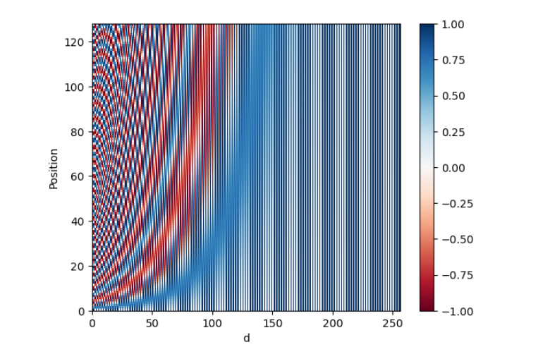
Each row represents a positional encoding - notice how none of the rows are identical! You have created a unique positional encoding for each of the words.

Congratulations on finishing this Lab! Now you should have a better understanding of the positional encoding in the transformer and this will surely help you with this week’s assignment!

Keep it up!

Transformer Decoder

In this video you’ll build your own transformer
decoder model, which is also known as GPT2. Once you know attention, it’s a fairly simple model as you’ll see, so let’s dive in. In this video, you’ll see the basic structure of
a transformer decoder. I’ll show you the definition of a transformer and how to implement the decoder and
the feed forward blocks. On the left you can see a picture of the
transformer decoder. As input, it gets a
tokenized sentence. A vector of integers as usual. The sentence gets embedded with word embeddings which
you know quite well by now. Then you add to these embeddings the
information about positions. This information is nothing else than learned vectors
representing 1, 2, 3 and so on up to some maximum length that
we’ll put into the model. The embedding of
the first word will get added with the
vector representing one. The embedding of the
second word with the vector representing
two, and so on. Now this constitutes the inputs for the first multi-headed
attention layer. After the attention layer, you have a feet-forward layer which operates on each
position independently. After each attention
and feet-forward layer, you put a residual
or skip connection. Just add the input
of that layer to its output and then perform
layer normalization. The attention and
feet-forward layers are repeated N times. The original model
started with N=6, but now transformers go
up to 100 or even more. Then you have a final
dense layer for output and a softmax
layer, and that’s it.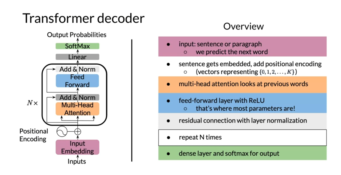

Now, don’t worry if you
didn’t catch it all at once. We’ll go through the structure again and with code to
explain all the detail. Here you’ll see the core
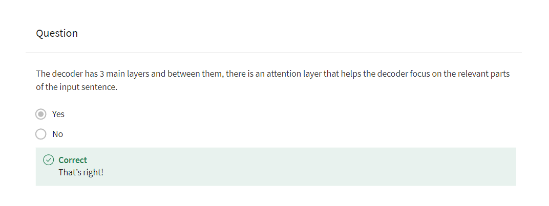
of the transformer model. It has three layers
at the beginning. Then the shift right, just introduces the start token, which your model will use
to predict the next word, you have the embedding which trains a word to
vector embedding. Positional encoding which
trains the vectors for one, two and so on, as
explained before. If the input to the model was tensor of shape a
batch by length, then after the embedding layer, it will be a tensor of shape batch by
length by d model. Where d model is the
size of these embeddings, and they usually
go to 512, 1,024. Nowadays, up to 10K or more. After these early layers, you’ll get N decoder blocks. Then a fully
connected layer that outputs tensors
of shape batch by length by vocab size and a log softmax for
cross-entropy loss.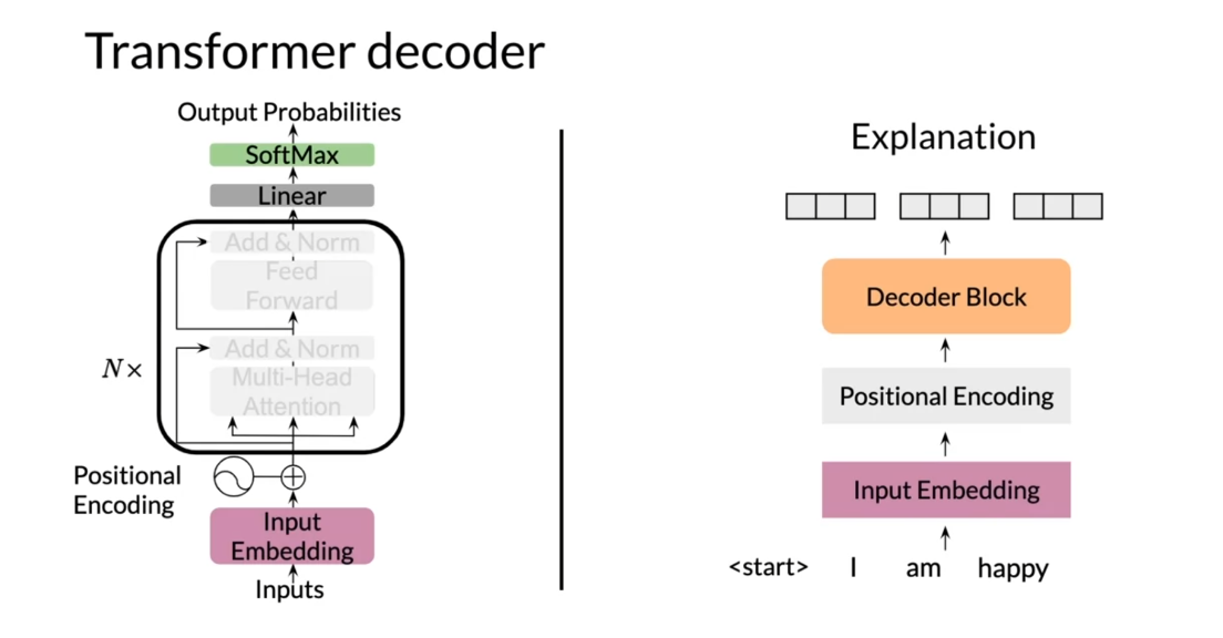

Let’s see how the
decoder block is built. It starts with a set of
vectors as an input sequence which are added to the corresponding
positional coding vectors, producing the so-called
positional input embedding. After embedding,
the input sequence passes through a multi-headed
attention model. While this model
processes each word, each position in
the input sequence, the attention itself
searches other positions in the sequence to help
identify relationships. Each of the words in the
sequence is weighted. Then in each layer of attention, there is a residual connection
around it followed by a layer normalization
step to speed up the training and significantly reduce the overall
processing time. Then each word is passed
through a feed-forward layer that is embeddings are fed
into a neural network. Then you have a dropout at the end as a form
of regularization. Next, a layer normalization step is applied, and the entire decoder block is repeated to a total of capital N times. Finally, the decoder
layer output is obtained.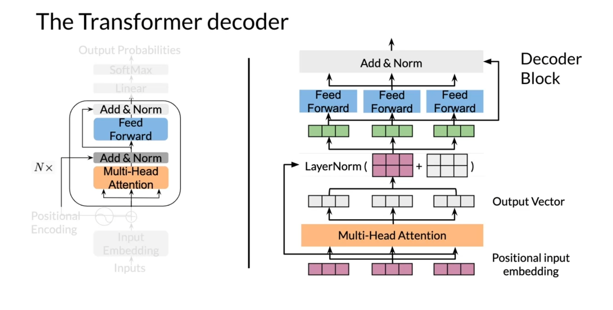

After mechanism and the
normalization step, some non linear transformations are introduced by including fully connected
feed forward layers with simple but non linear
low activation functions. For each inputs and you have shared parameters
for efficiency. The feed forward neural
network output vectors will essentially replace
the hidden states of the original RNN decoder.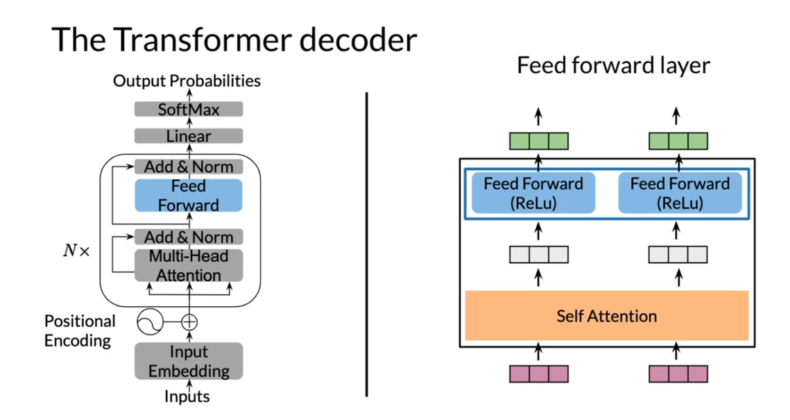

Let us recap what you
have seen in this video. You saw the building
blocks used to implement a transformer decoder. You saw that it
has three layers. It also has a module to
calculates a log softmax, which makes use of the
cross-entropy loss. You also saw the decoder
and the feet forward loss. You have now built your own
first transformer model. Congratulations. Wouldn’t it be nice
to see it in action?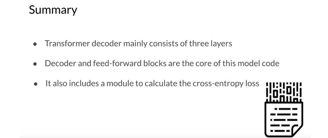

Transformer Summarizer

I’ll show you how to make a
summarizer. Let’s dive in. First I’ll show you
a brief overview of the transformer model code. Then you’ll see some
technical details about the data processing
for summarization. At the end of this video, you’ll see how to make inferences
with a language model. First, take a look
at the problem you will solve in this
week’s assignment. As input, you get
whole news articles. As output, your model is expected to produce the
summary of the articles, that is, few sentences that mention the most
important ideas. To do this, you’ll use the transformer model that I showed you in previous videos. But one thing may immediately
stand out to you. Transformer only takes text as input and predicts
the next word. For summarization, it turns out you just need to
concatenate the input, in this case the article, and put the summary after
it. Let me show you how. Here’s an example of how to
create input features for training the transformer from
an article and its summary. The input for the model is a long text that starts
with a news article, then comes the EOS tag, the summary, and then
another EOS tag. As usual, the input is tokenized as a
sequence of integers. Here, zero denotes padding, and one EOS, and all other numbers for the
tokens for different words. When you’re on the
transformer on this input, it will predict the next word by looking at all
the previous ones. But you do not want to
have a huge loss in the model just because it’s not able to predict
the correct ones. That’s why you have to
use a weighted loss. Instead of averaging the loss for every word in
the whole sequence, you weight the
loss for the words within the article with zeros, and the ones within
the summary with ones so the model only
focuses on the summary. However, when there is little
data for the summaries, it actually helps to weight the article loss with
non zero numbers, say 0.2 or 0.5 or even one. That way, the model is able to learn word relationships
that are common in the news. You will not have to do it
for this week’s assignment. But it’s good that
you have this in mind for your own applications.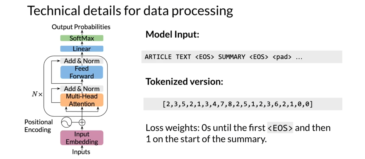

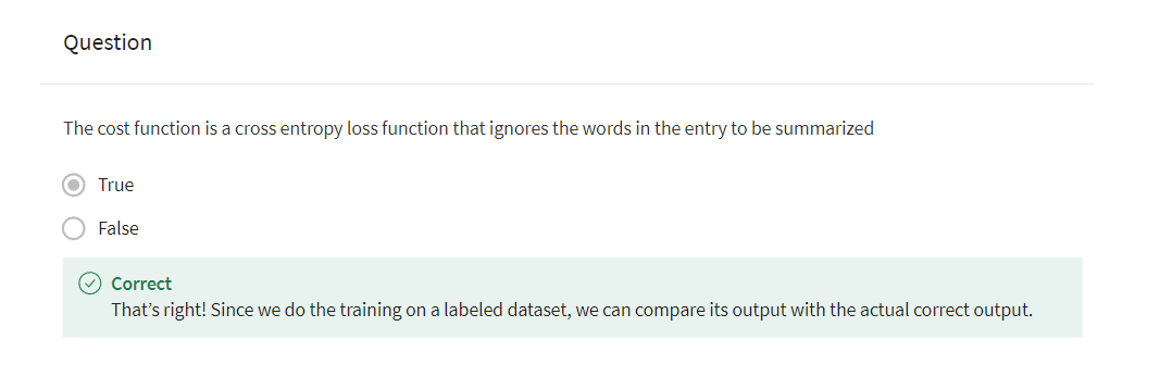
Another way to look at
what I discussed in the previous slide is by
looking at the cost function, which sums the losses
over the words J within the summary for every
example I in the batch. The cost function is a
cross entropy function that ignores the words from
the article to be summarized.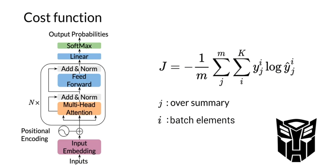

Now that you know
how to construct the inputs and the model, you can train your
transformer summarizer. Recall again that
transformers predict the next word and your
input is in use article. At test or inference time, you will input the
article with the EOS token to the model and
ask for the next word. It is the first word
of the summary. Then you will ask
for the next word, and the next, and so on, until you get the EOS token. When you run your
transformer model, it generates a
probability distribution over all possible words. You will sample from
this distribution so each time you
run this process, you’ll get a different summary. I think you’ll have
fun experimenting with this in the
coding exercise.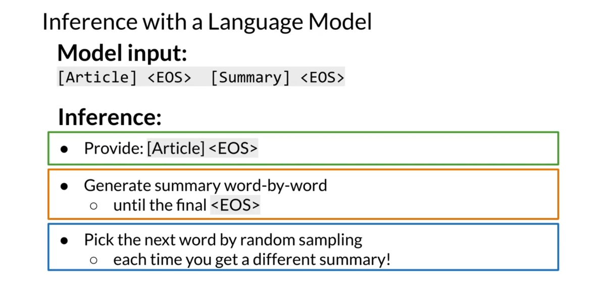

In this video, you
saw how to implement a transformer decoder
for summarization. As a key point, the
model aims to optimize a weighted cross
entropy function that focuses on the summary. The summarization
task is basically text generation where the
whole article is input. This week you have learned how to build your
own transformer, and you have used it to
create a summarizer. I hope you enjoyed the journey. Transformer is a
really powerful model that is not hard to understand. Next week, I’ll show you how
to get even better results. You’ll use a more
powerful version of transformer with pre
training. Don’t miss it.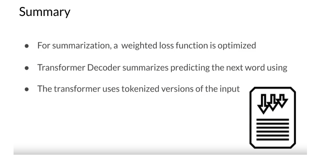

Quiz: Text Summarization

第四题改正：

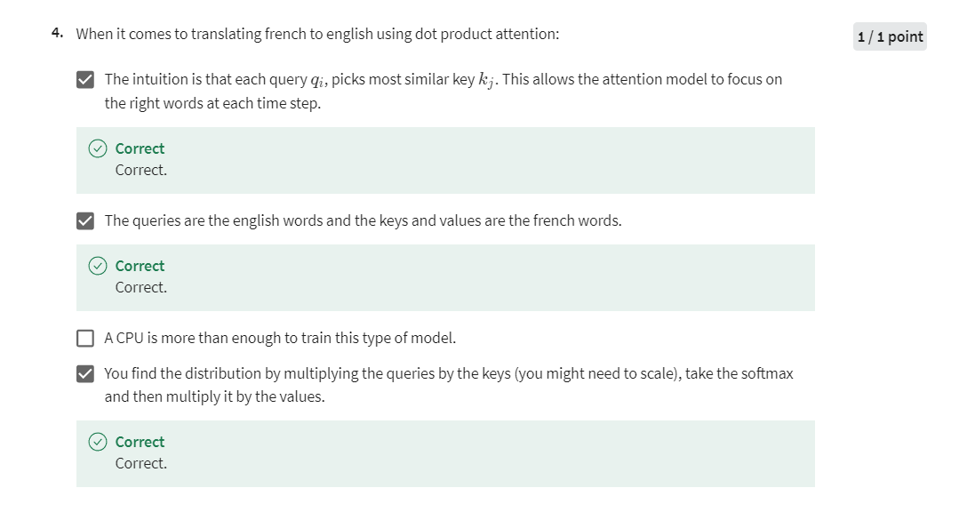
在注意力机制中，query 表示当前要翻译的目标语言（英语）的单词，而 keys 和 values 表示源语言（法语）的单词。通过计算 query 和每个 key 的相似度，然后将这些相似度作为权重来对 values 进行加权求和，就可以得到翻译后的目标语言单词。因此，在法语到英语的翻译中，应该将法语单词作为 keys 和 values，将英语单词作为 queries。

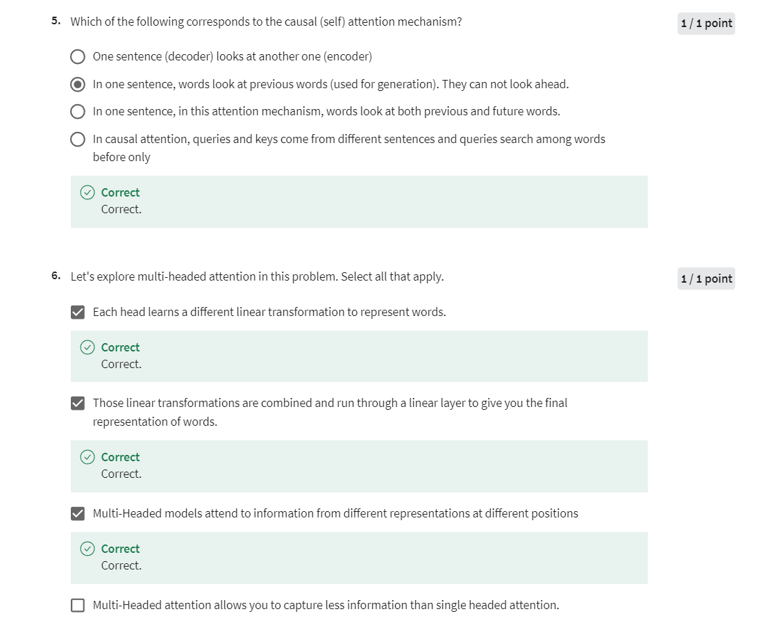
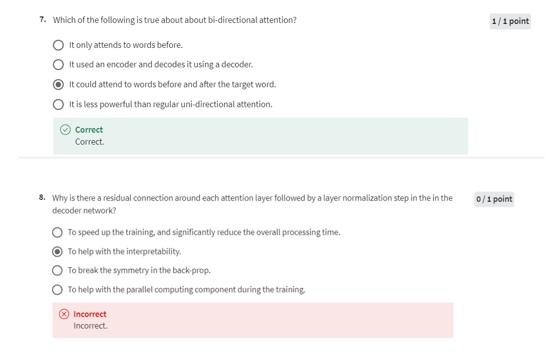
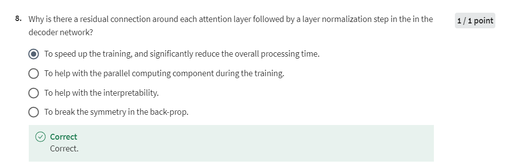
第八题改正：残差连接的好处是加速训练

Programming Assignment: Transformer Summarizer

Assignment 2: Transformer Summarizer

Welcome to the second assignment of course 4. In this assignment you will explore summarization using the transformer model. Yes, you will implement the transformer decoder from scratch, but we will slowly walk you through it. There are many hints in this notebook so feel free to use them as needed. Actually by the end of this notebook you will have implemented the full transformer (both encoder and decoder) but you will only be graded on the implementation of the decoder as the encoder is provided for you.

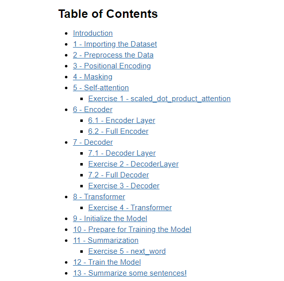
Introduction

Summarization is an important task in natural language processing and could be useful for a consumer enterprise. For example, bots can be used to scrape articles, summarize them, and then you can use sentiment analysis to identify the sentiment about certain stocks. Who wants to read an article or a long email today anyway, when you can build a transformer to summarize text for you? Let’s get started. By completing this assignment you will learn to:

• Use built-in functions to preprocess your data
• Implement DotProductAttention
• Implement Causal Attention
• Understand how attention works
• Build the transformer model
• Evaluate your model
• Summarize an article

As you can tell, this model is slightly different than the ones you have already implemented. This is heavily based on attention and does not rely on sequences, which allows for parallel computing.

import os
os.environ['TF_CPP_MIN_LOG_LEVEL'] = '3'

import numpy as np
import pandas as pd
import tensorflow as tf
import matplotlib.pyplot as plt
import time
import utils

import textwrap
wrapper = textwrap.TextWrapper(width=70)

tf.keras.utils.set_random_seed(10)

import w2_unittest
1
2
3
4
5
6
7
8
9
10
11
12
13
14
15
16

1 - Import the Dataset

You have the dataset saved in a .json file, which you can easily open with pandas. The loading function has already been taken care of in utils.py.

data_dir = "data/corpus"

train_data, test_data = utils.get_train_test_data(data_dir)

# Take one example from the dataset and print it
example_summary, example_dialogue = train_data.iloc[10]
print(f"Dialogue:\n{example_dialogue}")
print(f"\nSummary:\n{example_summary}")
1
2
3
4
5
6
7
8

Output

Dialogue:
Lucas: Hey! How was your day?
Demi: Hey there! 
Demi: It was pretty fine, actually, thank you!
Demi: I just got promoted! :D
Lucas: Whoa! Great news!
Lucas: Congratulations!
Lucas: Such a success has to be celebrated.
Demi: I agree! :D
Demi: Tonight at Death & Co.?
Lucas: Sure!
Lucas: See you there at 10pm?
Demi: Yeah! See you there! :D

Summary:
Demi got promoted. She will celebrate that with Lucas at Death & Co at 10 pm.
1
2
3
4
5
6
7
8
9
10
11
12
13
14
15
16

2 - Preprocess the data

First you will do some preprocessing of the data and split it into inputs and outputs. Here you also remove some of the characters that are specific to this dataset and add the [EOS] (end of sentence) token to the end, like it was discussed in the lecture videos. You will also add a [SOS] (start of sentence) token to the beginning of the sentences.

document, summary = utils.preprocess(train_data)
document_test, summary_test = utils.preprocess(test_data)
1
2

utils.py文件如下

import pandas as pd
import re


def get_train_test_data(data_dir):
    # Get the train data
    train_data = pd.read_json(f"{data_dir}/train.json")
    train_data.drop(['id'], axis=1, inplace=True)

    # Get the test data
    test_data = pd.read_json(f"{data_dir}/test.json")
    test_data.drop(['id'], axis=1, inplace=True)
    
    return train_data, test_data


def preprocess(input_data):
    # Define the custom preprocessing function
    def preprocess_util(input_data):
        # Convert all text to lowercase
        lowercase = input_data.lower()
        # Remove newlines and double spaces
        removed_newlines = re.sub("\n|\r|\t", " ",  lowercase)
        removed_double_spaces = ' '.join(removed_newlines.split(' '))
        # Add start of sentence and end of sentence tokens
        s = '[SOS] ' + removed_double_spaces + ' [EOS]'
        return s
    
    # Apply the preprocessing to the train and test datasets
    input_data['summary'] = input_data.apply(lambda row : preprocess_util(row['summary']), axis = 1)
    input_data['dialogue'] = input_data.apply(lambda row : preprocess_util(row['dialogue']), axis = 1)

    document = input_data['dialogue']
    summary = input_data['summary']
    
    return document, summary

1
2
3
4
5
6
7
8
9
10
11
12
13
14
15
16
17
18
19
20
21
22
23
24
25
26
27
28
29
30
31
32
33
34
35
36
37

Now perform the standard preprocessing with the tensorflow library. You will need to modify the filters, because you dont want the [EOS] tokens to be removed.

Then create the vocabulary by combining the data in the documents and the summaries and using .fit_on_texts():

# The [ and ] from default tokens cannot be removed, because they mark the SOS and EOS token.
filters = '!"#$%&()*+,-./:;<=>?@\\^_`{|}~\t\n'
oov_token = '[UNK]'

tokenizer = tf.keras.preprocessing.text.Tokenizer(filters=filters, oov_token=oov_token, lower=False)

documents_and_summary = pd.concat([document, summary], ignore_index=True)

tokenizer.fit_on_texts(documents_and_summary)

inputs = tokenizer.texts_to_sequences(document)
targets = tokenizer.texts_to_sequences(summary)

vocab_size = len(tokenizer.word_index) + 1

print(f'Size of vocabulary: {vocab_size}')
1
2
3
4
5
6
7
8
9
10
11
12
13
14
15
16

Output

Size of vocabulary: 34250
1

Now you can pad the tokenized sequences for the training data.

For the purpose of this notebook you need to limit the length of the sequences, as transformers are really big models and are not meant to be trained in such small environments.

# Limit the size of the input and output data for being able to run it in this environment.
encoder_maxlen = 150
decoder_maxlen = 50

# Pad the sequences.
inputs = tf.keras.preprocessing.sequence.pad_sequences(inputs, maxlen=encoder_maxlen, padding='post', truncating='post')
targets = tf.keras.preprocessing.sequence.pad_sequences(targets, maxlen=decoder_maxlen, padding='post', truncating='post')

inputs = tf.cast(inputs, dtype=tf.int32)
targets = tf.cast(targets, dtype=tf.int32)

# Create the final training dataset.
BUFFER_SIZE = 10000
BATCH_SIZE = 64

dataset = tf.data.Dataset.from_tensor_slices((inputs, targets)).shuffle(BUFFER_SIZE).batch(BATCH_SIZE)
1
2
3
4
5
6
7
8
9
10
11
12
13
14
15
16

3 - Positional Encoding

In sequence to sequence tasks, the relative order of your data is extremely important to its meaning. When you were training sequential neural networks such as RNNs, you fed your inputs into the network in order. Information about the order of your data was automatically fed into your model. However, when you train a Transformer network using multi-head attention, you feed your data into the model all at once. While this dramatically reduces training time, there is no information about the order of your data. This is where positional encoding is useful.

You have learned how to implement the positional encoding in one of this week’s labs. Here you will use the positional_encoding function to create positional encodings for your transformer. The function is already implemented for you.

def positional_encoding(positions, d_model):
    """
    Precomputes a matrix with all the positional encodings 
    
    Arguments:
        positions (int): Maximum number of positions to be encoded 
        d_model (int): Encoding size 
    
    Returns:
        pos_encoding (tf.Tensor): A matrix of shape (1, position, d_model) with the positional encodings
    """
    
    position = np.arange(positions)[:, np.newaxis]
    k = np.arange(d_model)[np.newaxis, :]
    i = k // 2
    
    # initialize a matrix angle_rads of all the angles 
    angle_rates = 1 / np.power(10000, (2 * i) / np.float32(d_model))
    angle_rads = position * angle_rates
  
    # apply sin to even indices in the array; 2i
    angle_rads[:, 0::2] = np.sin(angle_rads[:, 0::2])
  
    # apply cos to odd indices in the array; 2i+1
    angle_rads[:, 1::2] = np.cos(angle_rads[:, 1::2])
    
    pos_encoding = angle_rads[np.newaxis, ...]
    
    return tf.cast(pos_encoding, dtype=tf.float32)
1
2
3
4
5
6
7
8
9
10
11
12
13
14
15
16
17
18
19
20
21
22
23
24
25
26
27
28
29

4 - Masking

There are two types of masks that are useful when building your Transformer network: the padding mask and the look-ahead mask. Both help the softmax computation give the appropriate weights to the words in your input sentence.

You have already learned how to implement and use them in one of this week’s labs. Here they are implemented for you.

def create_padding_mask(decoder_token_ids):
    """
    Creates a matrix mask for the padding cells
    
    Arguments:
        decoder_token_ids (matrix like): matrix of size (n, m)
    
    Returns:
        mask (tf.Tensor): binary tensor of size (n, 1, m)
    """    
    seq = 1 - tf.cast(tf.math.equal(decoder_token_ids, 0), tf.float32)
  
    # add extra dimensions to add the padding to the attention logits. 
    # this will allow for broadcasting later when comparing sequences
    return seq[:, tf.newaxis, :] 


def create_look_ahead_mask(sequence_length):
    """
    Returns a lower triangular matrix filled with ones
    
    Arguments:
        sequence_length (int): matrix size
    
    Returns:
        mask (tf.Tensor): binary tensor of size (sequence_length, sequence_length)
    """
    mask = tf.linalg.band_part(tf.ones((1, sequence_length, sequence_length)), -1, 0)
    return mask 
1
2
3
4
5
6
7
8
9
10
11
12
13
14
15
16
17
18
19
20
21
22
23
24
25
26
27
28
29

5 - Self-Attention

As the authors of the Transformers paper state, “Attention is All You Need”.

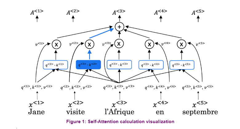
The use of self-attention paired with traditional convolutional networks allows for parallelization which speeds up training. You will implement scaled dot product attention which takes in a query, key, value, and a mask as inputs to return rich, attention-based vector representations of the words in your sequence. This type of self-attention can be mathematically expressed as:
$$\text{ Attention }(Q,K,V)=\mathrm{softmax}\left(\frac{Q{K}^T}{\sqrt{d_k}}+M\right)V\text{\hspace{1em}(4)}$$

• $Q$ is the matrix of queries
• $K$ is the matrix of keys
• $V$ is the matrix of values
• $M$ is the optional mask you choose to apply
• $d_k$ is the dimension of the keys, which is used to scale everything down so the softmax doesn’t explode

Exercise 1 - scaled_dot_product_attention

Implement the function scaled_dot_product_attention() to create attention-based representations.

Reminder: The boolean mask parameter can be passed in as none or as either padding or look-ahead.

• Multiply (1. - mask) by -1e9 before adding it to the scaled attention logits.

Additional Hints

• You may find tf.matmul useful for matrix multiplication (check how you can use the parameter transpose_b).
• You can use tf.keras.activations.softmax for softmax.

# GRADED FUNCTION: scaled_dot_product_attention
def scaled_dot_product_attention(q, k, v, mask):
    """
    Calculate the attention weights.
      q, k, v must have matching leading dimensions.
      k, v must have matching penultimate dimension, i.e.: seq_len_k = seq_len_v.
      The mask has different shapes depending on its type(padding or look ahead) 
      but it must be broadcastable for addition.

    Arguments:
        q (tf.Tensor): query of shape (..., seq_len_q, depth)
        k (tf.Tensor): key of shape (..., seq_len_k, depth)
        v (tf.Tensor): value of shape (..., seq_len_v, depth_v)
        mask (tf.Tensor): mask with shape broadcastable 
              to (..., seq_len_q, seq_len_k). Defaults to None.

    Returns:
        output -- attention_weights
    """
    ### START CODE HERE ###
    
    # Multiply q and k transposed.
    matmul_qk = tf.matmul(q, k, transpose_b=True)

    # scale matmul_qk with the square root of dk
    dk = tf.cast(tf.shape(k)[-1], tf.float32)
    scaled_attention_logits = matmul_qk / tf.math.sqrt(dk)

    # add the mask to the scaled tensor.
    if mask is not None:  # Don't replace this None
        scaled_attention_logits += (1. - mask) * (-1e9)

    # softmax is normalized on the last axis (seq_len_k) so that the scores add up to 1.
    attention_weights = tf.keras.activations.softmax(scaled_attention_logits)

    # Multiply the attention weights by v
    output = tf.matmul(attention_weights, v)
    
    ### END CODE HERE ###

    return output, attention_weights
1
2
3
4
5
6
7
8
9
10
11
12
13
14
15
16
17
18
19
20
21
22
23
24
25
26
27
28
29
30
31
32
33
34
35
36
37
38
39
40
41

# Test your function!
q = np.array([[1, 1, 0, 1], [0, 1, 1, 1], [1, 0, 1, 1]]).astype(np.float32)
k = np.array([[1, 1, 0, 1], [1, 0, 1, 1 ], [1, 1, 1, 0], [0, 0, 0, 1], [0, 1, 0, 1]]).astype(np.float32)
v = np.array([[0, 0], [1, 0], [1, 0], [1, 1], [1, 1]]).astype(np.float32)
mask = np.array([[[0, 1, 0, 1, 1], [1, 0, 0, 1, 1], [1, 1, 0, 1, 1]]])

ou, atw = scaled_dot_product_attention(q, k, v, mask)
ou = np.around(ou, decimals=2)
atw = np.around(atw, decimals=2)

print(f"Output:\n {ou}")
print(f"\nAttention weigths:\n {atw}")
1
2
3
4
5
6
7
8
9
10
11
12

Output

Output:
 [[[1.   0.62]
  [0.62 0.62]
  [0.74 0.31]]]

Attention weigths:
 [[[0.   0.38 0.   0.23 0.38]
  [0.38 0.   0.   0.23 0.38]
  [0.26 0.43 0.   0.16 0.16]]]
1
2
3
4
5
6
7
8
9

Expected Output

Output:
 [[[1.   0.62]
  [0.62 0.62]
  [0.74 0.31]]]

Attention weigths:
 [[[0.   0.38 0.   0.23 0.38]
  [0.38 0.   0.   0.23 0.38]
  [0.26 0.43 0.   0.16 0.16]]]
1
2
3
4
5
6
7
8
9

# UNIT TEST
w2_unittest.test_scaled_dot_product_attention(scaled_dot_product_attention)
1
2

Output

 All tests passed!
1

Excellent work! You can now implement self-attention. With that, you can start building the encoder block!

6 - Encoder

The Transformer Encoder layer pairs self-attention and convolutional neural network style of processing to improve the speed of training and passes K and V matrices to the Decoder, which you’ll build later in the assignment. In this section of the assignment, you will implement the Encoder by pairing multi-head attention and a feed forward neural network (Figure 2a).

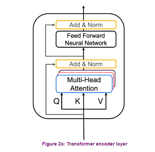
• MultiHeadAttention you can think of as computing the self-attention several times to detect different features.
• Feed forward neural network contains two Dense layers which we’ll implement as the function FullyConnected

Your input sentence first passes through a multi-head attention layer, where the encoder looks at other words in the input sentence as it encodes a specific word. The outputs of the multi-head attention layer are then fed to a feed forward neural network. The exact same feed forward network is independently applied to each position.

• For the MultiHeadAttention layer, you will use the MultiHeadAttention implemented in Keras. If you’re curious about how to split the query matrix Q, key matrix K, and value matrix V into different heads, you can look through the implementation.
• You will also use the Sequential API with two dense layers to built the feed forward neural network layers.

def FullyConnected(embedding_dim, fully_connected_dim):
    """
    Returns a sequential model consisting of two dense layers. The first dense layer has
    fully_connected_dim neurons and is activated by relu. The second dense layer has
    embedding_dim and no activation.

    Arguments:
        embedding_dim (int): output dimension
        fully_connected_dim (int): dimension of the hidden layer

    Returns:
        _ (tf.keras.Model): sequential model
    """
    return tf.keras.Sequential([
        tf.keras.layers.Dense(fully_connected_dim, activation='relu'),  # (batch_size, seq_len, d_model)
        tf.keras.layers.Dense(embedding_dim)  # (batch_size, seq_len, d_model)
    ])
1
2
3
4
5
6
7
8
9
10
11
12
13
14
15
16
17

6.1 Encoder Layer

Now you can pair multi-head attention and feed forward neural network together in an encoder layer! You will also use residual connections and layer normalization to help speed up training (Figure 2a).

The encoder block (Figure 2) is is already implemented for you. Take a very close look at its implementation, as you will later have to create the decoder yourself, and a lot of the code is very similar. The encoder block performs the following steps:

1. It takes the Q, V, K matrices and a boolean mask to a multi-head attention layer. Remember that to compute self-attention Q, V and K are the same. You will also perform Dropout in this multi-head attention layer during training.
2. There is a skip connection to add your original input x and the output of the multi-head attention layer.
3. After adding the skip connection, the output passes through the first normalization layer.
4. Finally, steps 1-3 are repeated but with the feed forward neural network with a dropout layer instead of the multi-head attention layer.

Additional Information (Click to expand)

• The __init__ method creates all the layers that will be accesed by the the call method. Wherever you want to use a layer defined inside the __init__ method you will have to use the syntax self.[insert layer name].
• You will find the documentation of MultiHeadAttention helpful. Note that if query, key and value are the same, then this function performs self-attention.
• The call arguments for self.mha are (Where B is for batch_size, T is for target sequence shapes, and S is output_shape):

• query: Query Tensor of shape (B, T, dim).
• value: Value Tensor of shape (B, S, dim).
• key: Optional key Tensor of shape (B, S, dim). If not given, will use the same value for both key and value, which is the most common case.
• attention_mask: a boolean mask of shape (B, T, S), that prevents attention to certain positions. The boolean mask specifies which query elements can attend to which key elements, 1 indicates attention and 0 indicates no attention. Broadcasting can happen for the missing batch dimensions and the head dimension.
• return_attention_scores: A boolean to indicate whether the output should be attention output if True, or (attention_output, attention_scores) if False. Defaults to False.
• training: Python boolean indicating whether the layer should behave in training mode (adding dropout) or in inference mode (no dropout). Defaults to either using the training mode of the parent layer/model, or False (inference) if there is no parent layer. Take a look at tf.keras.layers.Dropout for more details (Additional reading in Keras FAQ)

class EncoderLayer(tf.keras.layers.Layer):
    """
    The encoder layer is composed by a multi-head self-attention mechanism,
    followed by a simple, positionwise fully connected feed-forward network. 
    This architecture includes a residual connection around each of the two 
    sub-layers, followed by layer normalization.
    """
    def __init__(self, embedding_dim, num_heads, fully_connected_dim,
                 dropout_rate=0.1, layernorm_eps=1e-6):
        
        super(EncoderLayer, self).__init__()

        self.mha = tf.keras.layers.MultiHeadAttention(
            num_heads=num_heads,
            key_dim=embedding_dim,
            dropout=dropout_rate
        )

        self.ffn = FullyConnected(
            embedding_dim=embedding_dim,
            fully_connected_dim=fully_connected_dim
        )

        self.layernorm1 = tf.keras.layers.LayerNormalization(epsilon=layernorm_eps)
        self.layernorm2 = tf.keras.layers.LayerNormalization(epsilon=layernorm_eps)

        self.dropout_ffn = tf.keras.layers.Dropout(dropout_rate)
    
    def call(self, x, training, mask):
        """
        Forward pass for the Encoder Layer
        
        Arguments:
            x (tf.Tensor): Tensor of shape (batch_size, input_seq_len, fully_connected_dim)
            training (bool): Boolean, set to true to activate
                        the training mode for dropout layers
            mask (tf.Tensor): Boolean mask to ensure that the padding is not 
                    treated as part of the input
        Returns:
            encoder_layer_out (tf.Tensor): Tensor of shape (batch_size, input_seq_len, embedding_dim)
        """
        # calculate self-attention using mha(~1 line).
        # Dropout is added by Keras automatically if the dropout parameter is non-zero during training
        self_mha_output = self.mha(x, x, x, mask)  # Self attention (batch_size, input_seq_len, fully_connected_dim)
        
        # skip connection
        # apply layer normalization on sum of the input and the attention output to get the  
        # output of the multi-head attention layer
        skip_x_attention = self.layernorm1(x + self_mha_output)  # (batch_size, input_seq_len, fully_connected_dim)

        # pass the output of the multi-head attention layer through a ffn
        ffn_output = self.ffn(skip_x_attention)  # (batch_size, input_seq_len, fully_connected_dim)
        
        # apply dropout layer to ffn output during training
        # use `training=training`
        ffn_output = self.dropout_ffn(ffn_output, training=training)
        
        # apply layer normalization on sum of the output from multi-head attention (skip connection) and ffn output
        # to get the output of the encoder layer
        encoder_layer_out = self.layernorm2(skip_x_attention + ffn_output)  # (batch_size, input_seq_len, embedding_dim)
        
        return encoder_layer_out
    
1
2
3
4
5
6
7
8
9
10
11
12
13
14
15
16
17
18
19
20
21
22
23
24
25
26
27
28
29
30
31
32
33
34
35
36
37
38
39
40
41
42
43
44
45
46
47
48
49
50
51
52
53
54
55
56
57
58
59
60
61
62
63

6.2 - Full Encoder

Now you’re ready to build the full Transformer Encoder (Figure 2b), where you will embed your input and add the positional encodings you calculated. You will then feed your encoded embeddings to a stack of Encoder layers.

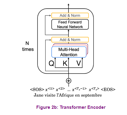
The Encoder class is implemented for you. It performs the following steps:

1. Pass the input through the Embedding layer.
2. Scale the embedding by multiplying it by the square root of the embedding dimension.
3. Add the position encoding: self.pos_encoding [:, :seq_len, :] to the embedding.
4. Pass the encoded embedding through a dropout layer
5. Pass the output of the dropout layer through the stack of encoding layers using a for loop.

class Encoder(tf.keras.layers.Layer):
    """
    The entire Encoder starts by passing the input to an embedding layer 
    and using positional encoding to then pass the output through a stack of
    encoder Layers
        
    """  
    def __init__(self, num_layers, embedding_dim, num_heads, fully_connected_dim, input_vocab_size,
               maximum_position_encoding, dropout_rate=0.1, layernorm_eps=1e-6):
        super(Encoder, self).__init__()

        self.embedding_dim = embedding_dim
        self.num_layers = num_layers

        self.embedding = tf.keras.layers.Embedding(input_vocab_size, self.embedding_dim)
        self.pos_encoding = positional_encoding(maximum_position_encoding, 
                                                self.embedding_dim)


        self.enc_layers = [EncoderLayer(embedding_dim=self.embedding_dim,
                                        num_heads=num_heads,
                                        fully_connected_dim=fully_connected_dim,
                                        dropout_rate=dropout_rate,
                                        layernorm_eps=layernorm_eps) 
                           for _ in range(self.num_layers)]

        self.dropout = tf.keras.layers.Dropout(dropout_rate)
        
    def call(self, x, training, mask):
        """
        Forward pass for the Encoder
        
        Arguments:
            x (tf.Tensor): Tensor of shape (batch_size, seq_len, embedding_dim)
            training (bool): Boolean, set to true to activate
                        the training mode for dropout layers
            mask (tf.Tensor): Boolean mask to ensure that the padding is not 
                    treated as part of the input

        Returns:
            x (tf.Tensor): Tensor of shape (batch_size, seq_len, embedding_dim)
        """
        seq_len = tf.shape(x)[1]
        
        # Pass input through the Embedding layer
        x = self.embedding(x)  # (batch_size, input_seq_len, embedding_dim)
        # Scale embedding by multiplying it by the square root of the embedding dimension
        x *= tf.math.sqrt(tf.cast(self.embedding_dim, tf.float32))
        # Add the position encoding to embedding
        x += self.pos_encoding[:, :seq_len, :]
        # Pass the encoded embedding through a dropout layer
        # use `training=training`
        x = self.dropout(x, training=training)
        # Pass the output through the stack of encoding layers 
        for i in range(self.num_layers):
            x = self.enc_layers[i](x, training, mask)

        return x  # (batch_size, input_seq_len, embedding_dim)
1
2
3
4
5
6
7
8
9
10
11
12
13
14
15
16
17
18
19
20
21
22
23
24
25
26
27
28
29
30
31
32
33
34
35
36
37
38
39
40
41
42
43
44
45
46
47
48
49
50
51
52
53
54
55
56
57
58

这里的 self.pos_encoding[:, :seq_len, :] 是对位置编码矩阵 self.pos_encoding 进行切片操作。具体来说：

• self.pos_encoding 是一个形状为 (1, maximum_position_encoding, embedding_dim) 的位置编码矩阵，其中 maximum_position_encoding 是要编码的最大位置数，embedding_dim 是词嵌入的维度。
• [:, :seq_len, :] 表示对矩阵进行切片操作，其中第一个 : 表示在第一个维度上取所有的值（因为此处第一个维度是 1，所以取所有值相当于取唯一的那个值），:seq_len 表示在第二个维度上取从第一个位置到第 seq_len 个位置的值，最后一个 : 表示在最后一个维度上取所有的值。

因此，self.pos_encoding[:, :seq_len, :] 的结果是一个形状为 (1, seq_len, embedding_dim) 的矩阵，包含了位置编码矩阵中从第一个位置到第 seq_len 个位置的位置编码向量。这样做是为了将位置编码与输入序列对应的词嵌入进行相加，以便在表示输入时考虑到位置信息。

7 - Decoder

Now it is time to implement the decoder. You have seen it in the videos and you can use some help by looking at the encoder implementation above. The Decoder layer takes the K and V matrices generated by the Encoder and computes the second multi-head attention layer with the Q matrix from the output (Figure 3a).

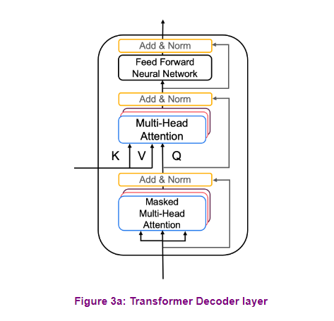
7.1 - Decoder Layer

Again, you’ll pair multi-head attention with a feed forward neural network, but this time you’ll implement two multi-head attention layers. You will also use residual connections and layer normalization to help speed up training (Figure 3a).

Exercise 2 - DecoderLayer

Implement DecoderLayer() using the call() method

1. Block 1 is a multi-head attention layer with a residual connection, and look-ahead mask. Like in the EncoderLayer, Dropout is defined within the multi-head attention layer.
2. Block 2 will take into account the output of the Encoder, so the multi-head attention layer will receive K and V from the encoder, and Q from the Block 1. You will then apply a normalization layer and a residual connection, just like you did before with the EncoderLayer.
3. Finally, Block 3 is a feed forward neural network with dropout and normalization layers and a residual connection.

Additional Hints:

• The first two blocks are fairly similar to the EncoderLayer except you will return attention_scores when computing self-attention

# GRADED FUNCTION: DecoderLayer
class DecoderLayer(tf.keras.layers.Layer):
    """
    The decoder layer is composed by two multi-head attention blocks, 
    one that takes the new input and uses self-attention, and the other 
    one that combines it with the output of the encoder, followed by a
    fully connected block. 
    """
    def __init__(self, embedding_dim, num_heads, fully_connected_dim, dropout_rate=0.1, layernorm_eps=1e-6):
        super(DecoderLayer, self).__init__()

        self.mha1 = tf.keras.layers.MultiHeadAttention(
            num_heads=num_heads,
            key_dim=embedding_dim,
            dropout=dropout_rate
        )

        self.mha2 = tf.keras.layers.MultiHeadAttention(
            num_heads=num_heads,
            key_dim=embedding_dim,
            dropout=dropout_rate
        )

        self.ffn = FullyConnected(
            embedding_dim=embedding_dim,
            fully_connected_dim=fully_connected_dim
        )

        self.layernorm1 = tf.keras.layers.LayerNormalization(epsilon=layernorm_eps)
        self.layernorm2 = tf.keras.layers.LayerNormalization(epsilon=layernorm_eps)
        self.layernorm3 = tf.keras.layers.LayerNormalization(epsilon=layernorm_eps)

        self.dropout_ffn = tf.keras.layers.Dropout(dropout_rate)
    
    def call(self, x, enc_output, training, look_ahead_mask, padding_mask):
        """
        Forward pass for the Decoder Layer
        
        Arguments:
            x (tf.Tensor): Tensor of shape (batch_size, target_seq_len, fully_connected_dim)
            enc_output (tf.Tensor): Tensor of shape(batch_size, input_seq_len, fully_connected_dim)
            training (bool): Boolean, set to true to activate
                        the training mode for dropout layers
            look_ahead_mask (tf.Tensor): Boolean mask for the target_input
            padding_mask (tf.Tensor): Boolean mask for the second multihead attention layer
        Returns:
            out3 (tf.Tensor): Tensor of shape (batch_size, target_seq_len, fully_connected_dim)
            attn_weights_block1 (tf.Tensor): Tensor of shape (batch_size, num_heads, target_seq_len, target_seq_len)
            attn_weights_block2 (tf.Tensor): Tensor of shape (batch_size, num_heads, target_seq_len, input_seq_len)
        """
        
        ### START CODE HERE ###
        # enc_output.shape == (batch_size, input_seq_len, fully_connected_dim)
        
        # BLOCK 1
        # calculate self-attention and return attention scores as attn_weights_block1.
        # Dropout will be applied during training (~1 line).
        mult_attn_out1, attn_weights_block1 = self.mha1(x, x, x, look_ahead_mask, return_attention_scores=True)
        
        # apply layer normalization (layernorm1) to the sum of the attention output and the input (~1 line)
        Q1 = self.layernorm1(mult_attn_out1 + x)

        # BLOCK 2
        # calculate self-attention using the Q from the first block and K and V from the encoder output. 
        # Dropout will be applied during training
        # Return attention scores as attn_weights_block2 (~1 line) 
        mult_attn_out2, attn_weights_block2 = self.mha2(Q1, enc_output, enc_output, padding_mask, return_attention_scores=True)
        
        # apply layer normalization (layernorm2) to the sum of the attention output and the output of the first block (~1 line)
        mult_attn_out2 = self.layernorm2(mult_attn_out2 + Q1)
                
        #BLOCK 3
        # pass the output of the second block through a ffn
        ffn_output = self.ffn(mult_attn_out2)
        
        # apply a dropout layer to the ffn output
        # use `training=training`
        ffn_output = self.dropout_ffn(ffn_output, training=training)
        
        # apply layer normalization (layernorm3) to the sum of the ffn output and the output of the second block
        out3 = self.layernorm3(ffn_output + mult_attn_out2)
        ### END CODE HERE ###

        return out3, attn_weights_block1, attn_weights_block2
    
1
2
3
4
5
6
7
8
9
10
11
12
13
14
15
16
17
18
19
20
21
22
23
24
25
26
27
28
29
30
31
32
33
34
35
36
37
38
39
40
41
42
43
44
45
46
47
48
49
50
51
52
53
54
55
56
57
58
59
60
61
62
63
64
65
66
67
68
69
70
71
72
73
74
75
76
77
78
79
80
81
82
83
84
85

# Test your function!
key_dim = 12
n_heads = 16

decoderLayer_test = DecoderLayer(embedding_dim=key_dim, num_heads=n_heads, fully_connected_dim=32)

q = np.ones((1, 15, key_dim))
encoder_test_output = tf.convert_to_tensor(np.random.rand(1, 7, 8))
look_ahead_mask = create_look_ahead_mask(q.shape[1])

out, attn_w_b1, attn_w_b2 = decoderLayer_test(q, encoder_test_output, False, look_ahead_mask, None)

print(f"Using embedding_dim={key_dim} and num_heads={n_heads}:\n")
print(f"q has shape:{q.shape}")
print(f"Output of encoder has shape:{encoder_test_output.shape}\n")

print(f"Output of decoder layer has shape:{out.shape}")
print(f"Att Weights Block 1 has shape:{attn_w_b1.shape}")
print(f"Att Weights Block 2 has shape:{attn_w_b2.shape}")
1
2
3
4
5
6
7
8
9
10
11
12
13
14
15
16
17
18
19

Output

Using embedding_dim=12 and num_heads=16:

q has shape:(1, 15, 12)
Output of encoder has shape:(1, 7, 8)

Output of decoder layer has shape:(1, 15, 12)
Att Weights Block 1 has shape:(1, 16, 15, 15)
Att Weights Block 2 has shape:(1, 16, 15, 7)
1
2
3
4
5
6
7
8

Expected Output

Output:
Using embedding_dim=12 and num_heads=16:

q has shape:(1, 15, 12)
Output of encoder has shape:(1, 7, 8)

Output of decoder layer has shape:(1, 15, 12)
Att Weights Block 1 has shape:(1, 16, 15, 15)
Att Weights Block 2 has shape:(1, 16, 15, 7)
1
2
3
4
5
6
7
8
9

# UNIT TEST
w2_unittest.test_decoderlayer(DecoderLayer, create_look_ahead_mask)
1
2

Output

All tests passed!
1

7.2 - Full Decoder

You’re almost there! Time to use your Decoder layer to build a full Transformer Decoder (Figure 3b). You will embed your output and add positional encodings. You will then feed your encoded embeddings to a stack of Decoder layers.

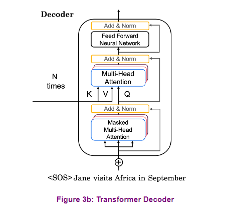
Exercise 3 - Decoder

Implement Decoder() using the call() method to embed your output, add positional encoding, and implement multiple decoder layers.

In this exercise, you will initialize your Decoder with an Embedding layer, positional encoding, and multiple DecoderLayers. Your call() method will perform the following steps:

1. Pass your generated output through the Embedding layer.
2. Scale your embedding by multiplying it by the square root of your embedding dimension. Remember to cast the embedding dimension to data type tf.float32 before computing the square root.
3. Add the position encoding: self.pos_encoding [:, :seq_len, :] to your embedding.
4. Pass the encoded embedding through a dropout layer, remembering to use the training parameter to set the model training mode.
5. Pass the output of the dropout layer through the stack of Decoding layers using a for loop.

# GRADED FUNCTION: Decoder
class Decoder(tf.keras.layers.Layer):
    """
    The entire Encoder starts by passing the target input to an embedding layer 
    and using positional encoding to then pass the output through a stack of
    decoder Layers
        
    """ 
    def __init__(self, num_layers, embedding_dim, num_heads, fully_connected_dim, target_vocab_size,
               maximum_position_encoding, dropout_rate=0.1, layernorm_eps=1e-6):
        super(Decoder, self).__init__()

        self.embedding_dim = embedding_dim
        self.num_layers = num_layers

        self.embedding = tf.keras.layers.Embedding(target_vocab_size, self.embedding_dim)
        self.pos_encoding = positional_encoding(maximum_position_encoding, self.embedding_dim)

        self.dec_layers = [DecoderLayer(embedding_dim=self.embedding_dim,
                                        num_heads=num_heads,
                                        fully_connected_dim=fully_connected_dim,
                                        dropout_rate=dropout_rate,
                                        layernorm_eps=layernorm_eps) 
                           for _ in range(self.num_layers)]
        self.dropout = tf.keras.layers.Dropout(dropout_rate)
    
    def call(self, x, enc_output, training, 
           look_ahead_mask, padding_mask):
        """
        Forward  pass for the Decoder
        
        Arguments:
            x (tf.Tensor): Tensor of shape (batch_size, target_seq_len, fully_connected_dim)
            enc_output (tf.Tensor):  Tensor of shape(batch_size, input_seq_len, fully_connected_dim)
            training (bool): Boolean, set to true to activate
                        the training mode for dropout layers
            look_ahead_mask (tf.Tensor): Boolean mask for the target_input
            padding_mask (tf.Tensor): Boolean mask for the second multihead attention layer
        Returns:
            x (tf.Tensor): Tensor of shape (batch_size, target_seq_len, fully_connected_dim)
            attention_weights (dict[str: tf.Tensor]): Dictionary of tensors containing all the attention weights
                                each of shape Tensor of shape (batch_size, num_heads, target_seq_len, input_seq_len)
        """

        seq_len = tf.shape(x)[1]
        attention_weights = {}
        
        ### START CODE HERE ###
        # create word embeddings 
        x = self.embedding(x)
        
        # scale embeddings by multiplying by the square root of their dimension
        x *= tf.math.sqrt(tf.cast(self.embedding_dim, tf.float32))
        
        # add positional encodings to word embedding
        x += self.pos_encoding[:, :seq_len, :]

        # apply a dropout layer to x
        # use `training=training`
        x = self.dropout(x, training=training)

        # use a for loop to pass x through a stack of decoder layers and update attention_weights (~4 lines total)
        for i in range(self.num_layers):
            # pass x and the encoder output through a stack of decoder layers and save the attention weights
            # of block 1 and 2 (~1 line)
            x, block1, block2 = self.dec_layers[i](x, enc_output, training, look_ahead_mask, padding_mask)

            #update attention_weights dictionary with the attention weights of block 1 and block 2
            attention_weights['decoder_layer{}_block1_self_att'.format(i+1)] = block1
            attention_weights['decoder_layer{}_block2_decenc_att'.format(i+1)] = block2
        ### END CODE HERE ###
        
        # x.shape == (batch_size, target_seq_len, fully_connected_dim)
        return x, attention_weights
1
2
3
4
5
6
7
8
9
10
11
12
13
14
15
16
17
18
19
20
21
22
23
24
25
26
27
28
29
30
31
32
33
34
35
36
37
38
39
40
41
42
43
44
45
46
47
48
49
50
51
52
53
54
55
56
57
58
59
60
61
62
63
64
65
66
67
68
69
70
71
72
73
74

# Test your function!
n_layers = 5
emb_d = 13
n_heads = 17
fully_connected_dim = 16
target_vocab_size = 300
maximum_position_encoding = 6

x = np.array([[3, 2, 1, 1], [2, 1, 1, 0], [2, 1, 1, 0]])

encoder_test_output = tf.convert_to_tensor(np.random.rand(3, 7, 9))

look_ahead_mask = create_look_ahead_mask(x.shape[1])

decoder_test = Decoder(n_layers, emb_d, n_heads, fully_connected_dim, target_vocab_size,maximum_position_encoding)
                   
outd, att_weights = decoder_test(x, encoder_test_output, False, look_ahead_mask, None)

print(f"Using num_layers={n_layers}, embedding_dim={emb_d} and num_heads={n_heads}:\n")
print(f"x has shape:{x.shape}")
print(f"Output of encoder has shape:{encoder_test_output.shape}\n")

print(f"Output of decoder has shape:{outd.shape}\n")
print("Attention weights:")
for name, tensor in att_weights.items():
    print(f"{name} has shape:{tensor.shape}")
1
2
3
4
5
6
7
8
9
10
11
12
13
14
15
16
17
18
19
20
21
22
23
24
25
26

Output

Using num_layers=5, embedding_dim=13 and num_heads=17:

x has shape:(3, 4)
Output of encoder has shape:(3, 7, 9)

Output of decoder has shape:(3, 4, 13)

Attention weights:
decoder_layer1_block1_self_att has shape:(3, 17, 4, 4)
decoder_layer1_block2_decenc_att has shape:(3, 17, 4, 7)
decoder_layer2_block1_self_att has shape:(3, 17, 4, 4)
decoder_layer2_block2_decenc_att has shape:(3, 17, 4, 7)
decoder_layer3_block1_self_att has shape:(3, 17, 4, 4)
decoder_layer3_block2_decenc_att has shape:(3, 17, 4, 7)
decoder_layer4_block1_self_att has shape:(3, 17, 4, 4)
decoder_layer4_block2_decenc_att has shape:(3, 17, 4, 7)
decoder_layer5_block1_self_att has shape:(3, 17, 4, 4)
decoder_layer5_block2_decenc_att has shape:(3, 17, 4, 7)
1
2
3
4
5
6
7
8
9
10
11
12
13
14
15
16
17
18

Expected Output

Using num_layers=5, embedding_dim=13 and num_heads=17:

x has shape:(3, 4)
Output of encoder has shape:(3, 7, 9)

Output of decoder has shape:(3, 4, 13)

Attention weights:
decoder_layer1_block1_self_att has shape:(3, 17, 4, 4)
decoder_layer1_block2_decenc_att has shape:(3, 17, 4, 7)
decoder_layer2_block1_self_att has shape:(3, 17, 4, 4)
decoder_layer2_block2_decenc_att has shape:(3, 17, 4, 7)
decoder_layer3_block1_self_att has shape:(3, 17, 4, 4)
decoder_layer3_block2_decenc_att has shape:(3, 17, 4, 7)
decoder_layer4_block1_self_att has shape:(3, 17, 4, 4)
decoder_layer4_block2_decenc_att has shape:(3, 17, 4, 7)
decoder_layer5_block1_self_att has shape:(3, 17, 4, 4)
decoder_layer5_block2_decenc_att has shape:(3, 17, 4, 7)
1
2
3
4
5
6
7
8
9
10
11
12
13
14
15
16
17
18

# UNIT TEST
w2_unittest.test_decoder(Decoder, create_look_ahead_mask, create_padding_mask)
1
2

Output

 All tests passed!
1

8 - Transformer

Phew! This has been quite the assignment! Congratulations! You’ve done all the hard work, now it’s time to put it all together.

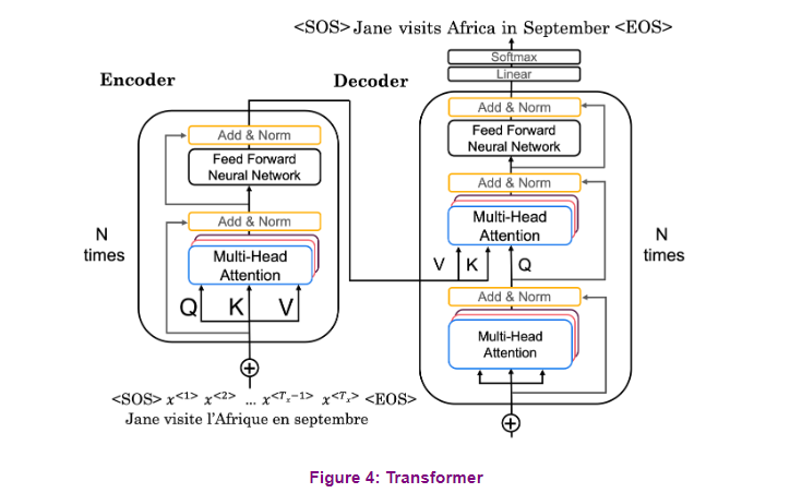
The flow of data through the Transformer Architecture is as follows:

• First your input passes through an Encoder, which is just repeated Encoder layers that you implemented:
  • embedding and positional encoding of your input
  • multi-head attention on your input
  • feed forward neural network to help detect features
• Then the predicted output passes through a Decoder, consisting of the decoder layers that you implemented:
  • embedding and positional encoding of the output
  • multi-head attention on your generated output
  • multi-head attention with the Q from the first multi-head attention layer and the K and V from the Encoder
  • a feed forward neural network to help detect features
• Finally, after the Nth Decoder layer, one dense layer and a softmax are applied to generate prediction for the next output in your sequence.

Exercise 4 - Transformer

Implement Transformer() using the call() method

1. Pass the input through the Encoder with the appropiate mask.
2. Pass the encoder output and the target through the Decoder with the appropiate mask.
3. Apply a linear transformation and a softmax to get a prediction.

# GRADED FUNCTION: Transformer
class Transformer(tf.keras.Model):
    """
    Complete transformer with an Encoder and a Decoder
    """
    def __init__(self, num_layers, embedding_dim, num_heads, fully_connected_dim, input_vocab_size, 
               target_vocab_size, max_positional_encoding_input,
               max_positional_encoding_target, dropout_rate=0.1, layernorm_eps=1e-6):
        super(Transformer, self).__init__()

        self.encoder = Encoder(num_layers=num_layers,
                               embedding_dim=embedding_dim,
                               num_heads=num_heads,
                               fully_connected_dim=fully_connected_dim,
                               input_vocab_size=input_vocab_size,
                               maximum_position_encoding=max_positional_encoding_input,
                               dropout_rate=dropout_rate,
                               layernorm_eps=layernorm_eps)

        self.decoder = Decoder(num_layers=num_layers, 
                               embedding_dim=embedding_dim,
                               num_heads=num_heads,
                               fully_connected_dim=fully_connected_dim,
                               target_vocab_size=target_vocab_size, 
                               maximum_position_encoding=max_positional_encoding_target,
                               dropout_rate=dropout_rate,
                               layernorm_eps=layernorm_eps)

        self.final_layer = tf.keras.layers.Dense(target_vocab_size, activation='softmax')
    
    def call(self, input_sentence, output_sentence, training, enc_padding_mask, look_ahead_mask, dec_padding_mask):
        """
        Forward pass for the entire Transformer
        Arguments:
            input_sentence (tf.Tensor): Tensor of shape (batch_size, input_seq_len, fully_connected_dim)
                              An array of the indexes of the words in the input sentence
            output_sentence (tf.Tensor): Tensor of shape (batch_size, target_seq_len, fully_connected_dim)
                              An array of the indexes of the words in the output sentence
            training (bool): Boolean, set to true to activate
                        the training mode for dropout layers
            enc_padding_mask (tf.Tensor): Boolean mask to ensure that the padding is not 
                    treated as part of the input
            look_ahead_mask (tf.Tensor): Boolean mask for the target_input
            dec_padding_mask (tf.Tensor): Boolean mask for the second multihead attention layer
        Returns:
            final_output (tf.Tensor): The final output of the model
            attention_weights (dict[str: tf.Tensor]): Dictionary of tensors containing all the attention weights for the decoder
                                each of shape Tensor of shape (batch_size, num_heads, target_seq_len, input_seq_len)
        
        """
        ### START CODE HERE ###
        # call self.encoder with the appropriate arguments to get the encoder output
        enc_output = self.encoder(input_sentence, training, enc_padding_mask)
        
        # call self.decoder with the appropriate arguments to get the decoder output
        # dec_output.shape == (batch_size, tar_seq_len, fully_connected_dim)
        dec_output, attention_weights = self.decoder(output_sentence, enc_output, training, look_ahead_mask, dec_padding_mask)
        
        # pass decoder output through a linear layer and softmax (~1 line)
        final_output = self.final_layer(dec_output)
        ### END CODE HERE ###

        return final_output, attention_weights
1
2
3
4
5
6
7
8
9
10
11
12
13
14
15
16
17
18
19
20
21
22
23
24
25
26
27
28
29
30
31
32
33
34
35
36
37
38
39
40
41
42
43
44
45
46
47
48
49
50
51
52
53
54
55
56
57
58
59
60
61
62
63

# Test your function!
n_layers = 3
emb_d = 13
n_heads = 17
fully_connected_dim = 8
input_vocab_size = 300
target_vocab_size = 350
max_positional_encoding_input = 12
max_positional_encoding_target = 12

transformer = Transformer(n_layers, 
    emb_d, 
    n_heads, 
    fully_connected_dim, 
    input_vocab_size, 
    target_vocab_size, 
    max_positional_encoding_input,
    max_positional_encoding_target)

# 0 is the padding value
sentence_a = np.array([[2, 3, 1, 3, 0, 0, 0]])
sentence_b = np.array([[1, 3, 4, 0, 0, 0, 0]])

enc_padding_mask = create_padding_mask(sentence_a)
dec_padding_mask = create_padding_mask(sentence_a)

look_ahead_mask = create_look_ahead_mask(sentence_a.shape[1])

test_summary, att_weights = transformer(
    sentence_a,
    sentence_b,
    False,
    enc_padding_mask,
    look_ahead_mask,
    dec_padding_mask
)

print(f"Using num_layers={n_layers}, target_vocab_size={target_vocab_size} and num_heads={n_heads}:\n")
print(f"sentence_a has shape:{sentence_a.shape}")
print(f"sentence_b has shape:{sentence_b.shape}")

print(f"\nOutput of transformer (summary) has shape:{test_summary.shape}\n")
print("Attention weights:")
for name, tensor in att_weights.items():
    print(f"{name} has shape:{tensor.shape}")
1
2
3
4
5
6
7
8
9
10
11
12
13
14
15
16
17
18
19
20
21
22
23
24
25
26
27
28
29
30
31
32
33
34
35
36
37
38
39
40
41
42
43
44
45

Output

Using num_layers=3, target_vocab_size=350 and num_heads=17:

sentence_a has shape:(1, 7)
sentence_b has shape:(1, 7)

Output of transformer (summary) has shape:(1, 7, 350)

Attention weights:
decoder_layer1_block1_self_att has shape:(1, 17, 7, 7)
decoder_layer1_block2_decenc_att has shape:(1, 17, 7, 7)
decoder_layer2_block1_self_att has shape:(1, 17, 7, 7)
decoder_layer2_block2_decenc_att has shape:(1, 17, 7, 7)
decoder_layer3_block1_self_att has shape:(1, 17, 7, 7)
decoder_layer3_block2_decenc_att has shape:(1, 17, 7, 7)
1
2
3
4
5
6
7
8
9
10
11
12
13
14

Expected Output

Using num_layers=3, target_vocab_size=350 and num_heads=17:

sentence_a has shape:(1, 7)
sentence_b has shape:(1, 7)

Output of transformer (summary) has shape:(1, 7, 350)

Attention weights:
decoder_layer1_block1_self_att has shape:(1, 17, 7, 7)
decoder_layer1_block2_decenc_att has shape:(1, 17, 7, 7)
decoder_layer2_block1_self_att has shape:(1, 17, 7, 7)
decoder_layer2_block2_decenc_att has shape:(1, 17, 7, 7)
decoder_layer3_block1_self_att has shape:(1, 17, 7, 7)
decoder_layer3_block2_decenc_att has shape:(1, 17, 7, 7)
1
2
3
4
5
6
7
8
9
10
11
12
13
14

# UNIT TEST
w2_unittest.test_transformer(Transformer, create_look_ahead_mask, create_padding_mask)
1
2

Output

 All tests passed!
1

9 - Initialize the Model

Now that you have defined the model, you can initialize and train it. First you can initialize the model with the parameters below. Note that generally these models are much larger and you are using a smaller version to fit this environment and to be able to train it in just a few minutes.

The base model described in the original Transformer paper used num_layers=6, embedding_dim=512, and fully_connected_dim=2048.

# Define the model parameters
num_layers = 2
embedding_dim = 128
fully_connected_dim = 128
num_heads = 2
positional_encoding_length = 256

# Initialize the model
transformer = Transformer(
    num_layers, 
    embedding_dim, 
    num_heads, 
    fully_connected_dim,
    vocab_size, 
    vocab_size, 
    positional_encoding_length, 
    positional_encoding_length,
)
1
2
3
4
5
6
7
8
9
10
11
12
13
14
15
16
17
18

10 - Prepare for Training the Model

The original transformer paper uses Adam optimizer with custom learning rate scheduling, which we define in the cell below. This was empirically shown to produce faster convergence.

class CustomSchedule(tf.keras.optimizers.schedules.LearningRateSchedule):
    def __init__(self, d_model, warmup_steps=4000):
        super(CustomSchedule, self).__init__()
        self.d_model = tf.cast(d_model, dtype=tf.float32)
        self.warmup_steps = warmup_steps
    
    def __call__(self, step):
        step = tf.cast(step, dtype=tf.float32)
        arg1 = tf.math.rsqrt(step)
        arg2 = step * (self.warmup_steps ** -1.5)

        return tf.math.rsqrt(self.d_model) * tf.math.minimum(arg1, arg2)

learning_rate = CustomSchedule(embedding_dim)

optimizer = tf.keras.optimizers.Adam(0.0002, beta_1=0.9, beta_2=0.98, epsilon=1e-9)
1
2
3
4
5
6
7
8
9
10
11
12
13
14
15
16

Below you can plot, how the custom learning rate looks like.

plt.plot(learning_rate(tf.range(40000, dtype=tf.float32)))
plt.ylabel('Learning Rate')
plt.xlabel('Train Step')
1
2
3

Output

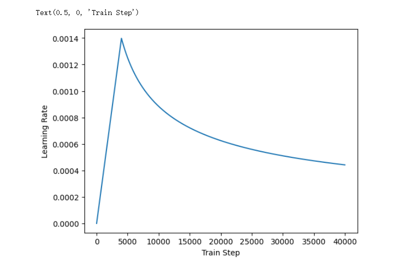
Next, you set up the loss. Since the target sequences are padded, it is important to apply a padding mask when calculating the loss.

You will use the sparse categorical cross-entropy loss function (tf.keras.losses.SparseCategoricalCrossentropy) and set the parameter from_logits to False since the Transformer does not output raw logits since the last layer has a softmax activation:

loss_object = tf.keras.losses.SparseCategoricalCrossentropy(from_logits=False, reduction='none')

def masked_loss(real, pred):
    mask = tf.math.logical_not(tf.math.equal(real, 0))
    loss_ = loss_object(real, pred)

    mask = tf.cast(mask, dtype=loss_.dtype)
    loss_ *= mask

    return tf.reduce_sum(loss_)/tf.reduce_sum(mask)


train_loss = tf.keras.metrics.Mean(name='train_loss')

# Here you will store the losses, so you can later plot them
losses = []
1
2
3
4
5
6
7
8
9
10
11
12
13
14
15
16

Now you can define your custom training function. If you are not very advanced with tensorflow, you can understand this function as an alternative to using model.compile() and model.fit(), but with added extra flexibility.

@tf.function
def train_step(model, inp, tar):
    """
    One training step for the transformer
    Arguments:
        inp (tf.Tensor): Input data to summarize
        tar (tf.Tensor): Target (summary)
    Returns:
        None
    """
    tar_inp = tar[:, :-1]
    tar_real = tar[:, 1:]

    # Create masks
    enc_padding_mask = create_padding_mask(inp)
    look_ahead_mask = create_look_ahead_mask(tf.shape(tar_inp)[1])
    dec_padding_mask = create_padding_mask(inp) # Notice that both encoder and decoder padding masks are equal

    with tf.GradientTape() as tape:
        predictions, _ = model(
            inp,
            tar_inp, 
            True, 
            enc_padding_mask, 
            look_ahead_mask, 
            dec_padding_mask
        )
        loss = masked_loss(tar_real, predictions)

    gradients = tape.gradient(loss, transformer.trainable_variables)    
    optimizer.apply_gradients(zip(gradients, transformer.trainable_variables))

    train_loss(loss)
1
2
3
4
5
6
7
8
9
10
11
12
13
14
15
16
17
18
19
20
21
22
23
24
25
26
27
28
29
30
31
32
33

Now you are ready for training the model. But before starting the training, you can also define one more set of functions to perform the inference. Because you are using a custom training loop, you can do whatever you want between the training steps. And wouldnt’t it be fun to see after each epoch some examples of how the model performs?

11 - Summarization

The last thing you will implement is inference. With this, you will be able to produce actual summaries of the documents. You will use a simple method called greedy decoding, which means you will predict one word at a time and append it to the output. You will start with an [SOS] token and repeat the word by word inference until the model returns you the [EOS] token or until you reach the maximum length of the sentence (you need to add this limit, otherwise a poorly trained model could give you infinite sentences without ever producing the [EOS] token.

Exercise 5 - next_word

Write a helper function that predicts the next word, so you can use it to write the whole sentences. Hint: this is very similar to what happens in the train_step, but you have to set the training of the model to False.

# GRADED FUNCTION: next_word
def next_word(model, encoder_input, output):
    """
    Helper function for summarization that uses the model to predict just the next word.
    Arguments:
        encoder_input (tf.Tensor): Input data to summarize
        output (tf.Tensor): (incomplete) target (summary)
    Returns:
        predicted_id (tf.Tensor): The id of the predicted word
    """
    ### START CODE HERE ###
    # Create a padding mask for the input (encoder)
    enc_padding_mask = create_padding_mask(encoder_input)
    # Create a look-ahead mask for the output
    look_ahead_mask = create_look_ahead_mask(tf.shape(output)[1])
    # Create a padding mask for the input (decoder)
    dec_padding_mask = create_padding_mask(encoder_input)

    # Run the prediction of the next word with the transformer model
    predictions, attention_weights = model(
        encoder_input,
        output,
        False,
        enc_padding_mask,
        look_ahead_mask,
        dec_padding_mask
    )
    ### END CODE HERE ###

    predictions = predictions[: ,-1:, :]
    predicted_id = tf.cast(tf.argmax(predictions, axis=-1), tf.int32)
    
    return predicted_id
1
2
3
4
5
6
7
8
9
10
11
12
13
14
15
16
17
18
19
20
21
22
23
24
25
26
27
28
29
30
31
32
33

Check if your function works.

# Take a random sentence as an input
input_document = tokenizer.texts_to_sequences(["a random sentence"])
input_document = tf.keras.preprocessing.sequence.pad_sequences(input_document, maxlen=encoder_maxlen, padding='post', truncating='post')
encoder_input = tf.expand_dims(input_document[0], 0)

# Take the start of sentence token as the only token in the output to predict the next word
output = tf.expand_dims([tokenizer.word_index["[SOS]"]], 0)

# predict the next word with your function
predicted_token = next_word(transformer, encoder_input, output)
print(f"Predicted token: {predicted_token}")

predicted_word = tokenizer.sequences_to_texts(predicted_token.numpy())[0]
print(f"Predicted word: {predicted_word}")
1
2
3
4
5
6
7
8
9
10
11
12
13
14

Output

Predicted token: [[14859]]
Predicted word: masses
1
2

Expected Output

Predicted token: [[14859]]
Predicted word: masses
1
2

# UNIT TEST
w2_unittest.test_next_word(next_word, transformer, encoder_input, output)
1
2

Output

 All tests passed!
1

def summarize(model, input_document):
    """
    A function for summarization using the transformer model
    Arguments:
        input_document (tf.Tensor): Input data to summarize
    Returns:
        _ (str): The summary of the input_document
    """    
    input_document = tokenizer.texts_to_sequences([input_document])
    input_document = tf.keras.preprocessing.sequence.pad_sequences(input_document, maxlen=encoder_maxlen, padding='post', truncating='post')
    encoder_input = tf.expand_dims(input_document[0], 0)
    
    output = tf.expand_dims([tokenizer.word_index["[SOS]"]], 0)
    
    for i in range(decoder_maxlen):
        predicted_id = next_word(model, encoder_input, output)
        output = tf.concat([output, predicted_id], axis=-1)
        
        if predicted_id == tokenizer.word_index["[EOS]"]:
            break

    return tokenizer.sequences_to_texts(output.numpy())[0]  # since there is just one translated document
1
2
3
4
5
6
7
8
9
10
11
12
13
14
15
16
17
18
19
20
21
22

Now you can already summarize a sentence! But beware, since the model was not yet trained at all, it will just produce nonsense.

training_set_example = 0

# Check a summary of a document from the training set
print('Training set example:')
print(document[training_set_example])
print('\nHuman written summary:')
print(summary[training_set_example])
print('\nModel written summary:')
summarize(transformer, document[training_set_example])
1
2
3
4
5
6
7
8
9

Output

Training set example:
[SOS] amanda: i baked  cookies. do you want some?  jerry: sure!  amanda: i'll bring you tomorrow :-) [EOS]

Human written summary:
[SOS] amanda baked cookies and will bring jerry some tomorrow. [EOS]

Model written summary:
"[SOS] masses kindergarten concept kindergarten concept bloomer wilingness sux sam kindergarten lisabeth kindergarten sawyer's sawyer's masses concept bloomer lisabeth bloomer wilingness 80000 bt hotsummer hoax hoax kieslowski wilingness 80000 dont't elis' 🐶❤️👍 cots saaaad evelynn inexperienced suji zubac forthcoming callum farmers extraordinary callum kindergarten worthy extraordinary readable 🐶❤️👍 thinkgn 🐶❤️👍 cots"
1
2
3
4
5
6
7
8

12 - Train the model

Now you can finally train the model. Below is a loop that will train your model for 20 epochs. note that it should take about 30 seconds per epoch (with the exception of the first few epochs which can take a few minutes each).

Note that after each epoch you perform the summarization on one of the sentences in the test set and print it out, so you can see how your model is improving.

# Take an example from the test set, to monitor it during training
test_example = 0
true_summary = summary_test[test_example]
true_document = document_test[test_example]

# Define the number of epochs
epochs = 20

# Training loop
for epoch in range(epochs):
    
    start = time.time()
    train_loss.reset_states()
    number_of_batches=len(list(enumerate(dataset)))

    for (batch, (inp, tar)) in enumerate(dataset):
        print(f'Epoch {epoch+1}, Batch {batch+1}/{number_of_batches}', end='\r')
        train_step(transformer, inp, tar)
    
    print (f'Epoch {epoch+1}, Loss {train_loss.result():.4f}')
    losses.append(train_loss.result())
    
    print (f'Time taken for one epoch: {time.time() - start} sec')
    print('Example summarization on the test set:')
    print('  True summarization:')
    print(f'    {true_summary}')
    print('  Predicted summarization:')
    print(f'    {summarize(transformer, true_document)}\n')
1
2
3
4
5
6
7
8
9
10
11
12
13
14
15
16
17
18
19
20
21
22
23
24
25
26
27
28

Output

Epoch 1, Loss 7.886631
Time taken for one epoch: 65.5023193359375 sec
Example summarization on the test set:
  True summarization:
    [SOS] hannah needs betty's number but amanda doesn't have it. she needs to contact larry. [EOS]
  Predicted summarization:
    [SOS] [EOS]

Epoch 2, Loss 6.599731
Time taken for one epoch: 26.72059965133667 sec
Example summarization on the test set:
  True summarization:
    [SOS] hannah needs betty's number but amanda doesn't have it. she needs to contact larry. [EOS]
  Predicted summarization:
    [SOS] is going to the the the the the the the the the the the the the the the the the the the the the the the the the the the the the the the the the the the the the the the the the the the the the the the

Epoch 3, Loss 6.028631
Time taken for one epoch: 19.050530433654785 sec
Example summarization on the test set:
  True summarization:
    [SOS] hannah needs betty's number but amanda doesn't have it. she needs to contact larry. [EOS]
  Predicted summarization:
    [SOS] tom is going to the new new new new new new new new new new new new new new new new new new new new new new new new new new new new new new new new new new new new new new new new new new new new new

Epoch 4, Loss 5.683631
Time taken for one epoch: 15.624465227127075 sec
Example summarization on the test set:
  True summarization:
    [SOS] hannah needs betty's number but amanda doesn't have it. she needs to contact larry. [EOS]
  Predicted summarization:
    [SOS] tom is going to the new new new new new new new new new new new new new new new job [EOS]

Epoch 5, Loss 5.475231
Time taken for one epoch: 15.841596603393555 sec
Example summarization on the test set:
  True summarization:
    [SOS] hannah needs betty's number but amanda doesn't have it. she needs to contact larry. [EOS]
  Predicted summarization:
    [SOS] the new new new new new new new job and she will be at the weekend [EOS]

Epoch 6, Loss 5.322431
Time taken for one epoch: 13.61079478263855 sec
Example summarization on the test set:
  True summarization:
    [SOS] hannah needs betty's number but amanda doesn't have it. she needs to contact larry. [EOS]
  Predicted summarization:
    [SOS] tom is going to the new job at the party [EOS]

Epoch 7, Loss 5.194831
Time taken for one epoch: 13.403933048248291 sec
Example summarization on the test set:
  True summarization:
    [SOS] hannah needs betty's number but amanda doesn't have it. she needs to contact larry. [EOS]
  Predicted summarization:
    [SOS] tom is going to the party with her [EOS]

Epoch 8, Loss 5.083231
Time taken for one epoch: 14.060023546218872 sec
Example summarization on the test set:
  True summarization:
    [SOS] hannah needs betty's number but amanda doesn't have it. she needs to contact larry. [EOS]
  Predicted summarization:
    [SOS] the new year's eve is going to the party [EOS]

Epoch 9, Loss 4.977331
Time taken for one epoch: 12.409761667251587 sec
Example summarization on the test set:
  True summarization:
    [SOS] hannah needs betty's number but amanda doesn't have it. she needs to contact larry. [EOS]
  Predicted summarization:
    [SOS] the new year's eve is going to the party [EOS]

Epoch 10, Loss 4.877331
Time taken for one epoch: 11.960368633270264 sec
Example summarization on the test set:
  True summarization:
    [SOS] hannah needs betty's number but amanda doesn't have it. she needs to contact larry. [EOS]
  Predicted summarization:
    [SOS] the car is going to the party with her [EOS]

Epoch 11, Loss 4.778031
Time taken for one epoch: 12.351112842559814 sec
Example summarization on the test set:
  True summarization:
    [SOS] hannah needs betty's number but amanda doesn't have it. she needs to contact larry. [EOS]
  Predicted summarization:
    [SOS] the car is going to the cinema with her [EOS]

Epoch 12, Loss 4.677431
Time taken for one epoch: 11.969927549362183 sec
Example summarization on the test set:
  True summarization:
    [SOS] hannah needs betty's number but amanda doesn't have it. she needs to contact larry. [EOS]
  Predicted summarization:
    [SOS] the car is going to the office today [EOS]

Epoch 13, Loss 4.574731
Time taken for one epoch: 11.802824974060059 sec
Example summarization on the test set:
  True summarization:
    [SOS] hannah needs betty's number but amanda doesn't have it. she needs to contact larry. [EOS]
  Predicted summarization:
    [SOS] jake will buy the dog for the office on the office [EOS]

Epoch 14, Loss 4.474431
Time taken for one epoch: 12.35073733329773 sec
Example summarization on the test set:
  True summarization:
    [SOS] hannah needs betty's number but amanda doesn't have it. she needs to contact larry. [EOS]
  Predicted summarization:
    [SOS] alice has sent a photo of the office today [EOS]

Epoch 15, Loss 4.372431
Time taken for one epoch: 12.06715440750122 sec
Example summarization on the test set:
  True summarization:
    [SOS] hannah needs betty's number but amanda doesn't have it. she needs to contact larry. [EOS]
  Predicted summarization:
    [SOS] alice and alice are going to the cinema with the store [EOS]

Epoch 16, Loss 4.271931
Time taken for one epoch: 11.935219764709473 sec
Example summarization on the test set:
  True summarization:
    [SOS] hannah needs betty's number but amanda doesn't have it. she needs to contact larry. [EOS]
  Predicted summarization:
    [SOS] hannah has just arrived to the office today because he has to go to the cinema with her [EOS]

Epoch 17, Loss 4.168931
Time taken for one epoch: 13.098976850509644 sec
Example summarization on the test set:
  True summarization:
    [SOS] hannah needs betty's number but amanda doesn't have it. she needs to contact larry. [EOS]
  Predicted summarization:
    [SOS] alice has just arrived to the cinema with her [EOS]

Epoch 18, Loss 4.074531
Time taken for one epoch: 11.558957576751709 sec
Example summarization on the test set:
  True summarization:
    [SOS] hannah needs betty's number but amanda doesn't have it. she needs to contact larry. [EOS]
  Predicted summarization:
    [SOS] hannah has just got the keys with alice and hannah and hannah are going to see it [EOS]

Epoch 19, Loss 3.971931
Time taken for one epoch: 11.799573183059692 sec
Example summarization on the test set:
  True summarization:
    [SOS] hannah needs betty's number but amanda doesn't have it. she needs to contact larry. [EOS]
  Predicted summarization:
    [SOS] alice has just finished the door for the wedding he has to go to the cinema with alice [EOS]

Epoch 20, Loss 3.880331
Time taken for one epoch: 11.239854097366333 sec
Example summarization on the test set:
  True summarization:
    [SOS] hannah needs betty's number but amanda doesn't have it. she needs to contact larry. [EOS]
  Predicted summarization:
    [SOS] alice has just finished the way to the cinema with amanda and hannah [EOS]
1
2
3
4
5
6
7
8
9
10
11
12
13
14
15
16
17
18
19
20
21
22
23
24
25
26
27
28
29
30
31
32
33
34
35
36
37
38
39
40
41
42
43
44
45
46
47
48
49
50
51
52
53
54
55
56
57
58
59
60
61
62
63
64
65
66
67
68
69
70
71
72
73
74
75
76
77
78
79
80
81
82
83
84
85
86
87
88
89
90
91
92
93
94
95
96
97
98
99
100
101
102
103
104
105
106
107
108
109
110
111
112
113
114
115
116
117
118
119
120
121
122
123
124
125
126
127
128
129
130
131
132
133
134
135
136
137
138
139
140
141
142
143
144
145
146
147
148
149
150
151
152
153
154
155
156
157
158
159

Plot the loss funtion.

plt.plot(losses)
plt.ylabel('Loss')
plt.xlabel('Epoch')
1
2
3

Output

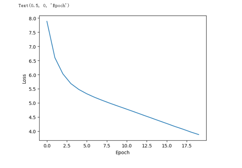
13 - Summarize some Sentences!

Below you can see an example of summarization of a sentence from the training set and a sentence from the test set. See if you notice anything interesting about them!

training_set_example = 0

# Check a summary of a document from the training set
print('Training set example:')
print(document[training_set_example])
print('\nHuman written summary:')
print(summary[training_set_example])
print('\nModel written summary:')
print(summarize(transformer, document[training_set_example]))
1
2
3
4
5
6
7
8
9

Output

Training set example:
[SOS] amanda: i baked  cookies. do you want some?  jerry: sure!  amanda: i'll bring you tomorrow :-) [EOS]

Human written summary:
[SOS] amanda baked cookies and will bring jerry some tomorrow. [EOS]

Model written summary:
[SOS] amanda will bring some cookies [EOS]
1
2
3
4
5
6
7
8

test_set_example = 3

# Check a summary of a document from the test set
print('Test set example:')
print(document_test[test_set_example])
print('\nHuman written summary:')
print(summary_test[test_set_example])
print('\nModel written summary:')
print(summarize(transformer, document_test[test_set_example]))
1
2
3
4
5
6
7
8
9

Output

Test set example:
[SOS] will: hey babe, what do you want for dinner tonight?  emma:  gah, don't even worry about it tonight  will: what do you mean? everything ok?  emma: not really, but it's ok, don't worry about cooking though, i'm not hungry  will: well what time will you be home?  emma: soon, hopefully  will: you sure? maybe you want me to pick you up?  emma: no no it's alright. i'll be home soon, i'll tell you when i get home.   will: alright, love you.   emma: love you too.  [EOS]

Human written summary:
[SOS] emma will be home soon and she will let will know. [EOS]

Model written summary:
[SOS] emma will pick up with emma at home tonight [EOS]
1
2
3
4
5
6
7
8

If you critically examine the output of the model, you can notice a few things:

• In the training set the model output is (almost) identical to the real output (already after 20 epochs and even more so with more epochs). This might be because the training set is relatively small and the model is relatively big and has thus learned the sentences in the training set by heart (overfitting).
• While the performance on the training set looks amazing, it is not so good on the test set. The model overfits, but fails to generalize. Again an easy candidate to blame is the small training set and a comparatively large model, but there might be a variety of other factors.
• Look at the test set example 3 and its summarization. Would you summarize it the same way as it is written here? Sometimes the data may be ambiguous. And the training of your model can only be as good as your data.

Here you only use a small dataset, to show that something can be learned in a reasonable amount of time in a relatively small environment. Generally, large transformers are trained on more than one task and on very large quantities of data to achieve superb performance. You will learn more about this in the rest of this course.

Congratulations on finishing this week’s assignment! You did a lot of work and now you should have a better understanding of the Transformers and their building blocks (encoder and decoder) and how they can be used for text summarization. And remember: you dont need to change much to use the same model for a translator, just change the dataset and it should work!

Keep it up!

Grades

后记

2024年3月31日花费1天的时间完成Week2的学习，重新学习了Transformer。之前使用PyTorch实现过Transformer，现在又用TensorFlow实现一遍Transformer，对它的结构更了解。同时对TF的语法越来越熟练。