Numpy 实现单层感知机对情感文本多分类

一、 实验题目

在给定文本数据集完成文本情感分类训练，在测试集完成测试，计算准确率

文本的特征可以使用TF或TF-IDF （可以使用sklearn库提取特征）设计合适的网络结构，选择合适的损失函数利用训练集完成网络训练，并在测试集上计算准确率。

训练集：train.txt

测试集: test.txt

二、 实验内容

1. 假定网络为单层感知机，且没有激活层，没有偏置，此时，网络输出为y=XW

2.设置损失函数为L_MSE，并随机初始化网络参数W

3.当满足终止条件时，终止优化，否则继续

4.计算网络输出y=XW，以及损失$$L_{MSE}=1/N(XW-Y{)}^T(XW-Y)$$

5.求导可得$\partial L_{MSE}/\partial W=1/N{X}^T(XW-Y)$

6.根据$W=W-\eta \partial L_{MSE}/\partial W$更新参数W

7.跳转到3

三、关键代码

from sklearn.feature_extraction.text import TfidfVectorizer
import numpy as np
from sklearn.preprocessing import LabelBinarizer
import matplotlib.pyplot as plt

train_set_path = 'train.txt'
test_set_path = 'test.txt'

'''
---------------Basic Concept---------------
1.   单层感知机 (输入层+输出层), 输入层为每个文本的特征值、输出层经过sigmoid函数, 为各类的预测值
2.   输入、输出、权重三者的关系为: Y = XW, 其中,X是(train_size, feature_size)的矩阵, W是(feature_size, class_num)的矩阵 
2.1. 需要注意的是, 由于输出经过了sigmoid函数, 因此值被限制在0～1之间, 而我们使用的标签是1~6的数, 所以要将它化成二进制码
3.   损失为L_MSE=1/N(XW−Y)^T(XW−Y) 对权重进行更新, 通过W = W - lr * ∂L_MSE/∂W, 其中∂L_MSE/∂W = 1/N X^T(XW−Y): [(feature_size, train_size) * (train_size, 6)]
3.1. 这里的Y是标签, 因为已经化成二进制值,所以每一个Yi是(1,6)的矩阵,如[0,0,0,1,0,0]表示标签4,

---------------END---------------

'''
# hyper parameters
learning_rate = 0.6
num_epochs = 4000
num_classes = 6
batch_size = 100
epochs = []
accur_train = []
accur_test = []


# 激活函数
def sigmoid(x):
    return 1 / (1 + np.exp(-x))


def dsigmoid(x):
    return x * (1 - x)


def data_process(path):
    '''
    :param path: 数据集路径
    :return: 文本、情感标签
    '''
    words = []
    data_set = []
    emotion = []
    with open(path, 'r') as F:
        line = F.readlines()
        for i in range(1, len(line)):
            emo = (int)(line[i].split()[1])  # 情感标签
            temp = line[i].split()[3:]
            out = ' '.join(temp)
            words.append(out)
            emotion.append(emo)
    return words, emotion


def tf_idf_cal(text):
    '''
    :param text: 待计算文本
    :return: 特征名称和特征值矩阵
    '''
    tf_idf_vec = TfidfVectorizer()
    tf_idf_matrix = tf_idf_vec.fit_transform(text)
    return tf_idf_vec.get_feature_names(), tf_idf_matrix.toarray()


words_train, emotion_train = data_process(train_set_path)
words_test, emotion_test = data_process(test_set_path)
train_feature_name, train_tf_idf = tf_idf_cal(words_train)
test_feature_name, test_tf_idf = tf_idf_cal(words_test)

# 处理训练集，将测试集特征在训练集中未出现过的特征值赋值为0
aligned_train_set = []
aligned_test_set = test_tf_idf
for k in range(len(train_tf_idf)):
    temp = []
    for i in range(len(test_feature_name)):
        feature = test_feature_name[i]
        if feature in train_feature_name:
            idx = train_feature_name.index(feature)
            temp.append(train_tf_idf[k][idx])
        else:
            temp.append(0)
    aligned_train_set.append(temp)


'''
方便查看：
---------------Basic Concept---------------
1.   单层感知机 (输入层+输出层), 输入层为每个文本的特征值、输出层经过sigmoid函数, 为各类的预测值
2.   输入、输出、权重三者的关系为: Y = XW, 其中,X是(train_size, feature_size)的矩阵, W是(feature_size, class_num)的矩阵 
2.1. 需要注意的是, 由于输出经过了sigmoid函数, 因此值被限制在0～1之间, 而我们使用的标签是1~6的数, 所以要将它化成二进制码
3.   损失为L_MSE=1/N(XW−Y)^T (XW−Y): [(6,train_size) * (train_size, 6)] 对权重进行更新, 通过W = W - lr * ∂L_MSE/∂W, 其中∂L_MSE/∂W = 1/N X^T(XW−Y): [(feature_size, train_size) * (train_size, 6)]
3.1. 这里的Y是标签, 因为已经化成二进制值,所以每一个Yi是(1,6)的矩阵,如[0,0,0,1,0,0]表示标签4,
     我们需要对Y进行扩展, 以便计算损失, 即将Y扩展成(train_size, 6)的矩阵,  

---------------END---------------

'''
def MSE(inputs, outputs, labels): # 这里的labels为(train_size, 6)的矩阵
    '''
    :param inputs: 特征矩阵 (train_size, feature_size)
    :param outputs: 网络输出 (train_size, num_class)
    :param labels: 标签 (train_size, num_class)
    :return: MES loss和它对W的偏导数
    '''
    n = outputs.shape[0] # train_size
    mse_loss = 0  # 所有样本的mse loss之和
    loss_mat = (outputs - labels) ** 2 / n  # 矩阵(train_size, train_size)
    for loss in loss_mat:
        mse_loss += loss.sum()
    loss_partial_mat = np.dot(inputs.T, (outputs - labels)) / n  # 矩阵(feature_size, num_class)
    return mse_loss, loss_partial_mat

'''
单层感知机
'''
class Perceptron:
    def __init__(self, in_size, out_size):
        self.in_size = in_size
        self.out_size = out_size
        self.weights = np.random.randn(in_size, out_size) # 随机化权重矩阵

    def forward(self, X):
        out = np.dot(X, self.weights)
        out = sigmoid(out)  # sigmoid函数，输出值被限制到0和1之间
        return out

# 转换成numpy数组
aligned_train_set = np.array(aligned_train_set)
aligned_test_set = np.array(aligned_test_set)
emotion_train = np.array(emotion_train)
emotion_test = np.array(emotion_test)

# 数值为1~6的情感标签转化成二进制
emotion_train_b = LabelBinarizer().fit_transform(emotion_train)
emotion_test_b = LabelBinarizer().fit_transform(emotion_test)

# 数据集参数
total_step = train_size = len(aligned_train_set)
test_size = len(aligned_test_set)
feature_size = len(aligned_train_set[0])



'''
Train the perceptron and Predict the label each batch
'''
perceptron = Perceptron(feature_size, num_classes)
for epoch in range(num_epochs):
    out = perceptron.forward(aligned_train_set)
    out_test = perceptron.forward(aligned_test_set)

    mse_loss, loss_partial_mat = MSE(aligned_train_set, out, emotion_train_b)
    perceptron.weights = perceptron.weights - learning_rate * loss_partial_mat
    if epoch % batch_size == 0:
        pre_label = []
        for i in range(out.shape[0]):
            pre_label.append(np.argmax(out[i]) + 1)
        accuracy = np.mean(np.equal(pre_label, emotion_train))
        print('Train_Set: Epoch [{}/{}], Loss: {:.4f}, Accuracy: {}'.format(epoch + 1, num_epochs, mse_loss,
                                                                            100 * accuracy))
        accur_train.append(100 * accuracy)

        pre_label = []
        for i in range(out_test.shape[0]):
            pre_label.append(np.argmax(out_test[i]) + 1)
        accuracy = np.mean(np.equal(pre_label, emotion_test))
        print('Test_Set: Epoch [{}/{}], Loss: {:.4f}, Accuracy: {}'.format(epoch + 1, num_epochs, mse_loss,
                                                                            100 * accuracy))
        epochs.append(epoch)
        accur_test.append(100 * accuracy)

plt.ylim((0, 100))
plt.xlabel("Epoch")
plt.ylabel("Accuracy")
plt.plot(epochs, accur_train, marker='o')
plt.plot(epochs, accur_test, marker='*')
plt.legend(['Train', 'test'])
plt.show()

1
2
3
4
5
6
7
8
9
10
11
12
13
14
15
16
17
18
19
20
21
22
23
24
25
26
27
28
29
30
31
32
33
34
35
36
37
38
39
40
41
42
43
44
45
46
47
48
49
50
51
52
53
54
55
56
57
58
59
60
61
62
63
64
65
66
67
68
69
70
71
72
73
74
75
76
77
78
79
80
81
82
83
84
85
86
87
88
89
90
91
92
93
94
95
96
97
98
99
100
101
102
103
104
105
106
107
108
109
110
111
112
113
114
115
116
117
118
119
120
121
122
123
124
125
126
127
128
129
130
131
132
133
134
135
136
137
138
139
140
141
142
143
144
145
146
147
148
149
150
151
152
153
154
155
156
157
158
159
160
161
162
163
164
165
166
167
168
169
170
171
172
173
174
175
176
177
178
179
180
181
182

四、实验结果：

通过numpy矩阵进行运算速度还是很快的，基本在几秒内就能够算出结果。

(1) Epoch 500

(2) Epoch 2000

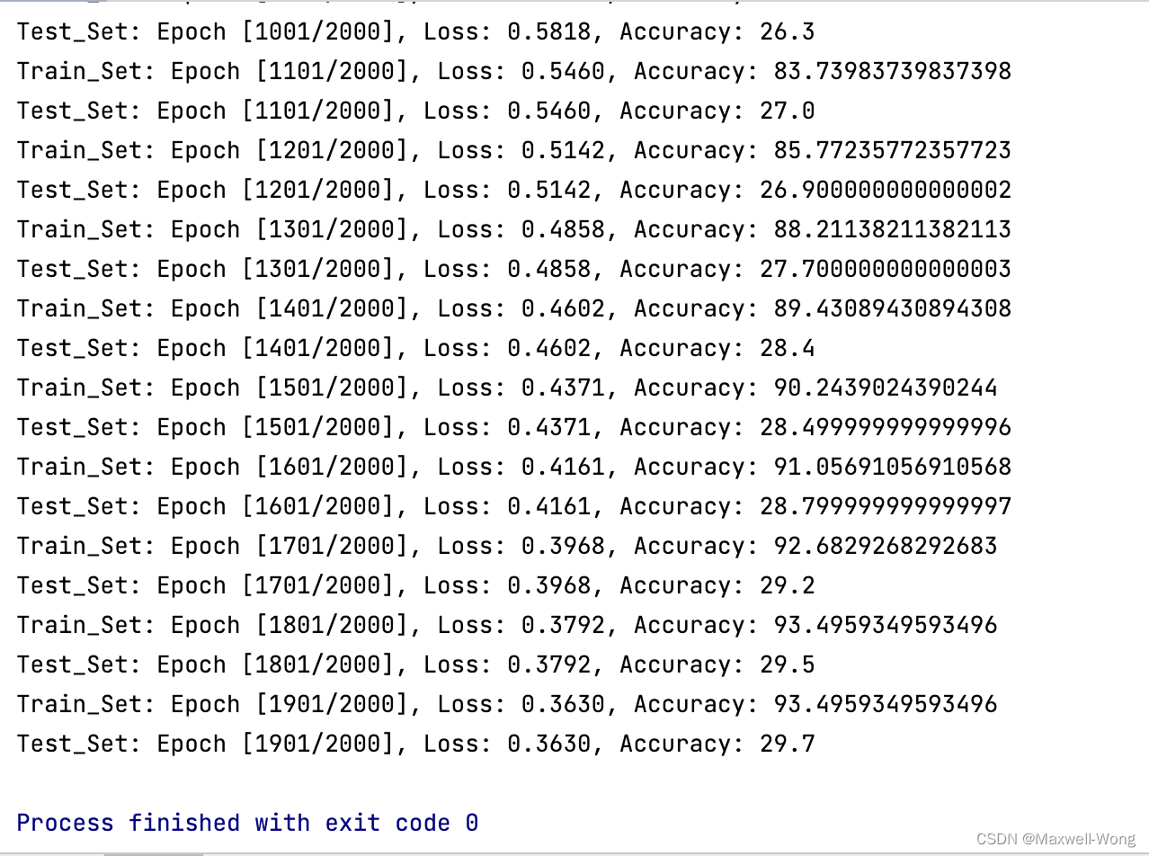
(3) Epoch 4000