[科研图像处理]用matlab平替image-j，有点麻烦，但很灵活！

做材料与生物相关方向的同学应该对image-j并不陌生，前几天有个师兄拜托我用image-j分析一些图片，但使用过后发现我由于不了解image-j的工作流程而对结果并不确信，而且image-j的功能无法拓展，对有些图片的处理效果并不好，因此我想到自己用matlab实现类似的功能，虽然没有友好的互动界面，但好在大家可以以此为基础，自己设计功能，更好得适配自己的研究方向。
测试文件与源程序下载地址，提取码: tcxa
视频教程（B站）

⏰：V1.0目前支持的功能：
😀：图像的开闭运算，分别对应分离细小连接与填充细小空洞
😀：二值化：支持单个自动阈值、单个手动阈值、手动区间阈值
😀：筛选颗粒：支持基于圆度筛选、基于面积大小筛选
😀：图像统计：支持颗粒占全图比例、图像真实面积、颗粒真实面积、颗粒数量统计

下载后设置好matlab的工作目录，

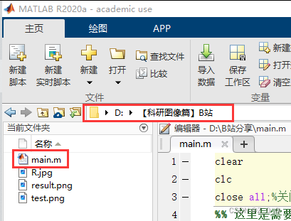
打开main.m文件开始使用，我把所有需要修改的地方都放在最前面：

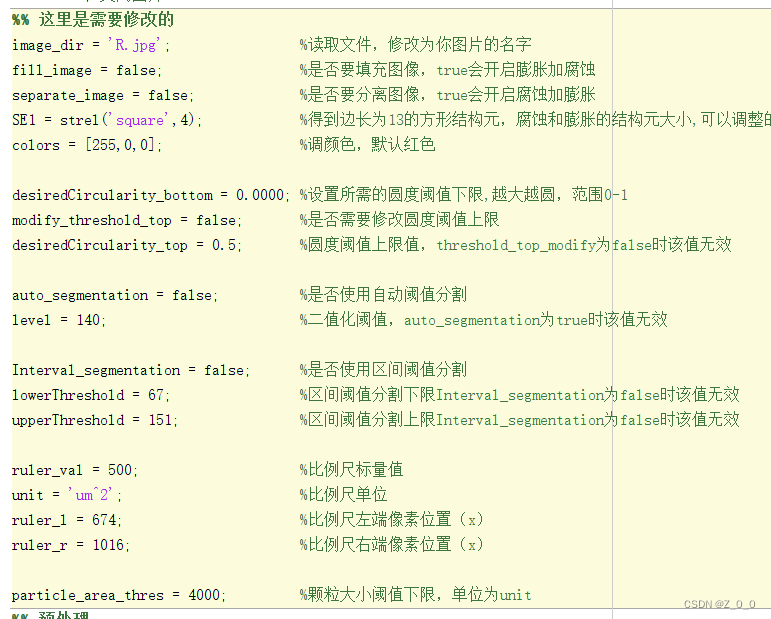
建议一开始使用测试图片的时候，对这两项做如下设置：

auto_segmentation = true;          %是否使用自动阈值分割
Interval_segmentation = false;      %是否使用区间阈值分割
1
2

完整代码

clear
clc
close all;%关闭图片
%% 这里是需要修改的
image_dir = 'test.png';             %读取文件，修改为你图片的名字
fill_image = false;                 %是否要填充图像，true会开启膨胀加腐蚀
separate_image = false;             %是否要分离图像，true会开启腐蚀加膨胀
SE1 = strel('square',8);            %得到边长为13的方形结构元，腐蚀和膨胀的结构元大小,可以调整的大小看看效果，点密集时候需要调整,dense_image为false时无效
colors = [0,255,0];                 %调颜色，默认红色

auto_segmentation = false;          %是否使用自动阈值分割
level = 200;                         %二值化阈值，auto_segmentation为true时该值无效

Interval_segmentation = false;      %是否使用区间阈值分割
lowerThreshold = 25;                %区间阈值分割下限Interval_segmentation为false时该值无效
upperThreshold = 61;                %区间阈值分割上限Interval_segmentation为false时该值无效

desiredCircularity_bottom = 0.0;    %设置所需的圆度阈值下限,越大越圆，范围0-1
modify_threshold_top = false;       %是否需要修改圆度阈值上限
desiredCircularity_top = 0.6;       %圆度阈值上限值，threshold_top_modify为false时该值无效

ruler_val = 50;                     %比例尺标量值
unit = 'um^2';                      %比例尺单位
ruler_l = 557;                      %比例尺左端像素位置（x）
ruler_r = 744;                      %比例尺右端像素位置（x）

particle_area_thres = 0;         %颗粒大小阈值下限，单位为unit
%% 预处理
imagetest1 = imread(image_dir);
imagetest_copy = imagetest1;
mysize=size(imagetest1);

if numel(mysize) == 2
  imagetest1 = cat(3,imagetest1,imagetest1,imagetest1); %将灰度图像转换为彩色图像
  imagetest_copy = cat(3,imagetest_copy,imagetest_copy,imagetest_copy);
end
imagetest1 = rgb2gray(imagetest1);
imagetest1_copy = imagetest1;

imshow(imagetest_copy)
impixelinfo%通过左下角的提示看比例尺坐标

%Filter = fspecial('average',[3,3]);

% gausFilter1 = fspecial('gaussian',[7,7],0.6);
% imagetest1 = imfilter(imagetest1,gausFilter1);
% imagetest_copy_Gau = imagetest1;

%imagetest_copy = rgb2gray(imagetest_copy);
%I2 = im2bw(imagetest1, 0.25);

if auto_segmentation
    fprintf(2,'注意你使用了自动阈值\n');
    level = graythresh(imagetest1); 
    imagetest1 = imbinarize(imagetest1, level);
elseif (~auto_segmentation&&~Interval_segmentation)
    fprintf(2,'注意你使用了手动阈值\n');
    imagetest1 = imbinarize(imagetest1, level/255);
end

if Interval_segmentation
    fprintf(2,'注意你使用了区间阈值\n');
    imagetest1 = (imagetest1_copy >= lowerThreshold) & (imagetest1_copy <= upperThreshold);%区间二值化
end
%% 腐蚀加膨胀
if fill_image
    fprintf(2,'注意你开启了填充\n')
    imagetest1 = imdilate(imagetest1,SE1);
    imagetest1 = imerode(imagetest1,SE1); 
end
if separate_image
    fprintf(2,'注意你开启了分离\n')
    imagetest1 = imerode(imagetest1,SE1); 
    imagetest1 = imdilate(imagetest1,SE1);
end
%% 圆度筛选封闭区域
labeledImage = bwlabel(imagetest1);%封闭空间标签
props = regionprops(labeledImage, 'Area', 'Perimeter');%实例化
circularity = (4 * pi * [props.Area]) ./ ([props.Perimeter].^2+0.0001);%求圆度

if ~modify_threshold_top
    desiredCircularity_top = max(circularity);% 设置所需的圆度阈值上限，一般不用动
end
selectedLabels = find((desiredCircularity_top > circularity) & (circularity> desiredCircularity_bottom));
selectedImage = ismember(labeledImage, selectedLabels);%根据圆度值做筛选
fprintf(2,['圆度阈值设置为:',num2str(desiredCircularity_bottom),'-',num2str(desiredCircularity_top),'\n']);
fprintf(2,['面积阈值设置为:',num2str(particle_area_thres),unit,'\n'])
%% 展示结果
figure
subplot(2,2,1);
%imshow(imagetest1);
imshow(imagetest_copy);%原图
subplot(2,2,2);
imhist(imagetest_copy)

subplot(2,2,3);
%imshow(imagetest_copy_Gau);
imshow(selectedImage);%展示筛选圆度之后的图像
%% 求解与图像结果美化
sum1 = sum(selectedImage(:));%求像素总数
m = size(imagetest_copy,1);
n = size(imagetest_copy,2);
sum2 = m * n;%原图总像素数
Proportion = sum1/sum2;%求比例
disp(['所选区域占全图的比例:',num2str(Proportion*100),'%'])
real_area = m * n * (ruler_val / (ruler_r - ruler_l))^2;
disp(['全图真实面积:',num2str(real_area),unit])
disp(['选区真实面积:',num2str(real_area*Proportion),unit])

R = imagetest_copy(:,:,1);
G = imagetest_copy(:,:,2);
B = imagetest_copy(:,:,3);

%默认红色
R(selectedImage)=colors(1);
G(selectedImage)=colors(2);      
B(selectedImage)=colors(3);
image_output=cat(3,R,G,B); 

% I = double(selectedImage).*double(I)
% image_output = imfuse(imagetest_copy,I)

subplot(2,2,4);
imshow(image_output)%原图与红色mask的叠加

image_output = uint8(image_output);
imwrite(image_output,'result.png')%保存

selectedImage_copy = selectedImage;%二值化图像
particle_area = regionprops(selectedImage_copy, 'Area');%实例化
disp(['颗粒总数（根据圆度筛选后）:',num2str(size(particle_area,1)),'个'])
particle_area_val = [particle_area.Area]*(ruler_val / (ruler_r - ruler_l))^2;%真实世界的面积

vector_particle = [];
for i= 1:size(particle_area_val,2)
    if particle_area_val(i) > particle_area_thres
        vector_particle = [vector_particle, particle_area_val(i)];
    end
end
labeledImage_2 = bwlabel(selectedImage_copy);%封闭空间标签
selectedLabels_2 = find(particle_area_val > particle_area_thres);
selectedImage_copy = ismember(labeledImage_2, selectedLabels_2);%根据面积做筛选

figure
imshow(selectedImage_copy)

mean_particle_real = mean(vector_particle);
disp(['根据面积筛选后颗粒个数:',num2str(size(selectedLabels_2,2))])
disp(['根据面积筛选后平均颗粒真实面积:',num2str(mean_particle_real),unit])
1
2
3
4
5
6
7
8
9
10
11
12
13
14
15
16
17
18
19
20
21
22
23
24
25
26
27
28
29
30
31
32
33
34
35
36
37
38
39
40
41
42
43
44
45
46
47
48
49
50
51
52
53
54
55
56
57
58
59
60
61
62
63
64
65
66
67
68
69
70
71
72
73
74
75
76
77
78
79
80
81
82
83
84
85
86
87
88
89
90
91
92
93
94
95
96
97
98
99
100
101
102
103
104
105
106
107
108
109
110
111
112
113
114
115
116
117
118
119
120
121
122
123
124
125
126
127
128
129
130
131
132
133
134
135
136
137
138
139
140
141
142
143
144
145
146
147
148
149