【python海洋专题九】Cartopy画地形等深线图

【python海洋专题九】Cartopy画地形等深线图

水深图基础差不多了，可以换成温度、盐度等

本期加上等深线

本期内容

1：地形等深线

cf = ax.contour(lon, lat, ele[:, :], levels=np.linspace(-9000,-100,10),colors='gray', linestyles='-',
                    linewidths=0.25, transform=ccrs.PlateCarree())
1
2

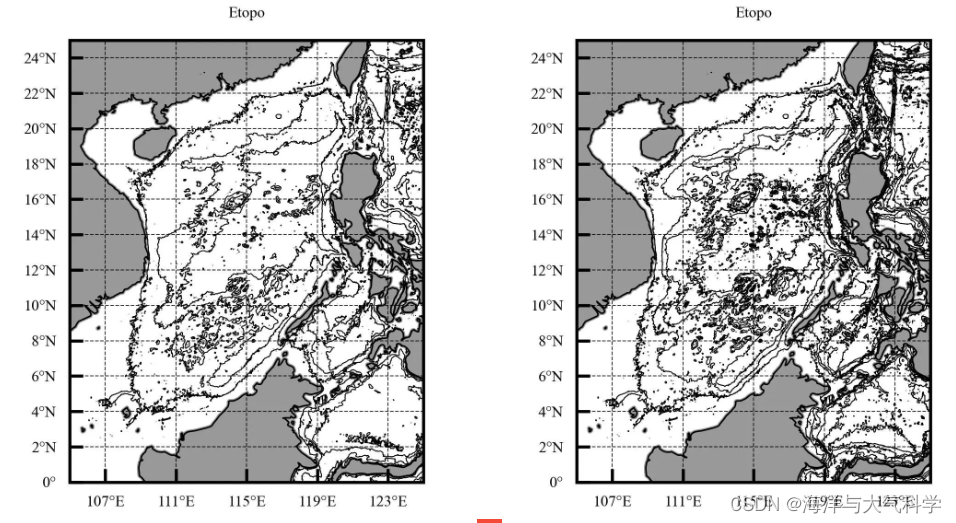
2：改变颜色

colors='gray'
1

3：改变粗细

linewidths=1，数字越大线条越粗。
1

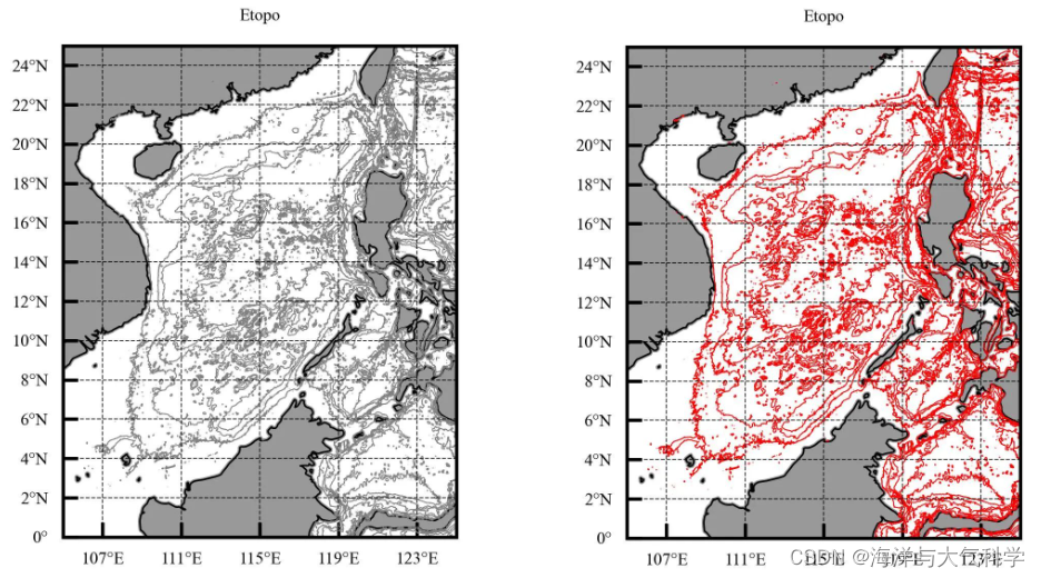
4：特定等值线

levels=[-9000, -8000, -5000, -3000, -1000, -300]；想画哪条，填写对应数字。
1

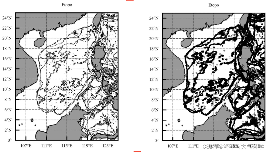
5：特定线条特定颜色和粗细

cf = ax.contour(lon, lat, ele[:, :], levels=[-8000,-6000,-4000,-2000,-200],colors='k', linestyles='-',
                    linewidths=0.3, transform=ccrs.PlateCarree())
cf = ax.contour(lon, lat, ele[:, :], levels=[-3000],colors='r', linestyles='-',
                    linewidths=0.5, transform=ccrs.PlateCarree())
1
2
3
4

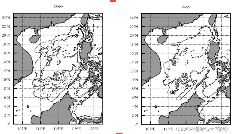
6：线条样式

linestyles='-.

图片
图片
图片
图片
图片

图片
7：显示数字

ax.clabel(cf,inline=True,fmt=‘%.f’,fontsize=3.5)
出现错误：不会了！

‘codes’ must be a 1D list or array with the same length of ‘vertices’. Your vertices have shape (2, 2) but your codes have shape (1,)

8：填充加上等值线

参考文献及其在本文中的作用

Python气象绘图笔记（五）——等高线 - 知乎 (zhihu.com)

【python海洋专题一】查看数据nc文件的属性并输出属性到txt文件

【python海洋专题二】读取水深nc文件并水深地形图
【python海洋专题三】图像修饰之画布和坐标轴

【Python海洋专题四】之水深地图图像修饰

【Python海洋专题五】之水深地形图海岸填充

【Python海洋专题六】之Cartopy画地形水深图

【python海洋专题】测试数据

【Python海洋专题七】Cartopy画地形水深图的陆地填充

【python海洋专题八】Cartopy画地形水深图的contourf填充间隔数调整

# -*- coding: utf-8 -*-
# %%
# Importing related function packages
import matplotlib.pyplot as plt
import cartopy.crs as ccrs
import cartopy.feature as feature
import numpy as np
import matplotlib.ticker as ticker
from cartopy import mpl
from cartopy.mpl.ticker import LongitudeFormatter, LatitudeFormatter
from cartopy.mpl.gridliner import LONGITUDE_FORMATTER, LATITUDE_FORMATTER
from matplotlib.font_manager import FontProperties
from netCDF4 import Dataset
from palettable.cmocean.diverging import Delta_4
from palettable.colorbrewer.sequential import GnBu_9
from palettable.colorbrewer.sequential import Blues_9
from palettable.scientific.diverging import Roma_20
from pylab import *
def reverse_colourmap(cmap, name='my_cmap_r'):
    reverse = []
    k = []

    for key in cmap._segmentdata:
        k.append(key)
        channel = cmap._segmentdata[key]
        data = []

        for t in channel:
            data.append((1 - t[0], t[2], t[1]))
        reverse.append(sorted(data))

    LinearL = dict(zip(k, reverse))
    my_cmap_r = mpl.colors.LinearSegmentedColormap(name, LinearL)
    return my_cmap_r

cmap = Blues_9.mpl_colormap
cmap_r = reverse_colourmap(cmap)
cmap1 = GnBu_9.mpl_colormap
cmap_r1 = reverse_colourmap(cmap1)
cmap2 = Roma_20.mpl_colormap
cmap_r2 = reverse_colourmap(cmap2)
# read data
a = Dataset('D:\pycharm_work\data\scs_etopo.nc')
print(a)
lon = a.variables['lon'][:]
lat = a.variables['lat'][:]
ele = a.variables['elevation'][:]
# 图三
# 设置地图全局属性
scale = '50m'
plt.rcParams['font.sans-serif'] = ['Times New Roman']  # 设置整体的字体为Times New Roman
fig = plt.figure(dpi=300, figsize=(3, 2), facecolor='w', edgecolor='blue')#设置一个画板，将其返还给fig
ax = fig.add_axes([0.05, 0.08, 0.92, 0.8], projection=ccrs.PlateCarree(central_longitude=180))
ax.set_extent([105, 125, 0, 25], crs=ccrs.PlateCarree())# 设置显示范围
land = feature.NaturalEarthFeature('physical', 'land', scale, edgecolor='face',
                                    facecolor=feature.COLORS['land'])
ax.add_feature(land, facecolor='0.6')
ax.add_feature(feature.COASTLINE.with_scale('50m'), lw=0.3)#添加海岸线：关键字lw设置线宽;linestyle设置线型
cs = ax.contourf(lon, lat, ele[:, :], levels=np.arange(-9000,0,20),extend='both',cmap=cmap_r1, transform=ccrs.PlateCarree())
# ------colorbar设置
cb = plt.colorbar(cs, ax=ax, extend='both', orientation='vertical',ticks=np.linspace(-9000, 0, 10))
cb.set_label('depth', fontsize=4, color='k')#设置colorbar的标签字体及其大小
cb.ax.tick_params(labelsize=4, direction='in') #设置colorbar刻度字体大小。
cf = ax.contour(lon, lat, ele[:, :], levels=[-5000,-2000,-500,-300,-100,-50,-10],colors='gray', linestyles='-',
                    linewidths=0.2,transform=ccrs.PlateCarree())
#ax.clabel(cf, inline=True, fontsize=8, colors='red', fmt='%1.0f',manual=False)

#ax.clabel(cf,inline=True,fmt='%.f',fontsize=3.5)

# 添加标题
ax.set_title('Etopo', fontsize=4)
# 利用Formatter格式化刻度标签
ax.set_xticks(np.arange(107, 125, 4), crs=ccrs.PlateCarree())#添加经纬度
ax.set_xticklabels(np.arange(107, 125, 4), fontsize=4)
ax.set_yticks(np.arange(0, 25, 2), crs=ccrs.PlateCarree())
ax.set_yticklabels(np.arange(0, 25, 2), fontsize=4)
ax.xaxis.set_major_formatter(LongitudeFormatter())
ax.yaxis.set_major_formatter(LatitudeFormatter())
ax.tick_params(color='k', direction='in')#更改刻度指向为朝内，颜色设置为蓝色
gl = ax.gridlines(crs=ccrs.PlateCarree(), draw_labels=False, xlocs=np.arange(107, 125, 4), ylocs=np.arange(0, 25, 2),
        linewidth=0.25, linestyle='--', color='k', alpha=0.8)#添加网格线
gl.top_labels, gl.bottom_labels, gl.right_labels, gl.left_labels = False, False, False, False
plt.savefig('scs_elevation1.jpg', dpi=600, bbox_inches='tight', pad_inches=0.1)  # 输出地图，并设置边框空白紧密
plt.show()
1
2
3
4
5
6
7
8
9
10
11
12
13
14
15
16
17
18
19
20
21
22
23
24
25
26
27
28
29
30
31
32
33
34
35
36
37
38
39
40
41
42
43
44
45
46
47
48
49
50
51
52
53
54
55
56
57
58
59
60
61
62
63
64
65
66
67
68
69
70
71
72
73
74
75
76
77
78
79
80
81
82
83
84
85