解析用户消费记录(数据分析三剑客综合使用)

博客地址：https://www.cnblogs.com/zylyehuo/

开发环境

• anaconda
  • 集成环境：集成好了数据分析和机器学习中所需要的全部环境
  • 安装目录不可以有中文和特殊符号
• jupyter
  • anaconda提供的一个基于浏览器的可视化开发工具

• 

import numpy as np
import pandas as pd
from pandas import DataFrame,Series
import matplotlib.pyplot as plt

第一部分：数据类型处理

• 数据加载
  • 字段含义：
    • user_id:用户ID
    • order_dt:购买日期
    • order_product:购买产品的数量
    • order_amount:购买金额
  • 观察数据
    • 查看数据的数据类型
    • 数据中是否存储在缺失值
    • 将order_dt转换成时间类型
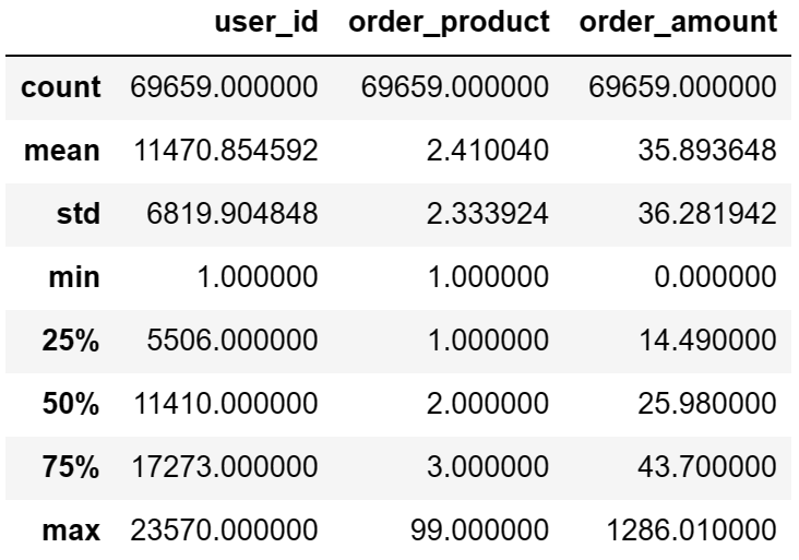
    • 查看数据的统计描述
      • 计算所有用户购买商品的平均数量
      • 计算所有用户购买商品的平均花费
    • 在源数据中添加一列表示月份:astype('datetime64[M]')

数据加载

• 设置字段：
  • user_id:用户ID
  • order_dt:购买日期
  • order_product:购买产品的数量
  • order_amount:购买金额

df = pd.read_csv('./data/CDNOW_master.txt',header=None,sep='\s+',names=['user_id','order_dt','order_product','order_amount'])
df

观察数据

• 查看数据的数据类型
• 数据中是否存储在缺失值

df.info()

<class 'pandas.core.frame.DataFrame'>
RangeIndex: 69659 entries, 0 to 69658
Data columns (total 4 columns):
 #   Column         Non-Null Count  Dtype  
---  ------         --------------  -----  
 0   user_id        69659 non-null  int64  
 1   order_dt       69659 non-null  int64  
 2   order_product  69659 non-null  int64  
 3   order_amount   69659 non-null  float64
dtypes: float64(1), int64(3)
memory usage: 2.1 MB

将order_dt转换成时间类型

df['order_dt'] = pd.to_datetime(df['order_dt'],format='%Y%m%d')
df.info()

<class 'pandas.core.frame.DataFrame'>
RangeIndex: 69659 entries, 0 to 69658
Data columns (total 4 columns):
 #   Column         Non-Null Count  Dtype         
---  ------         --------------  -----         
 0   user_id        69659 non-null  int64         
 1   order_dt       69659 non-null  datetime64[ns]
 2   order_product  69659 non-null  int64         
 3   order_amount   69659 non-null  float64       
dtypes: datetime64[ns](1), float64(1), int64(2)
memory usage: 2.1 MB

查看数据的统计描述

• 计算所有用户购买商品的平均数量
• 计算所有用户购买商品的平均花费

df.describe()

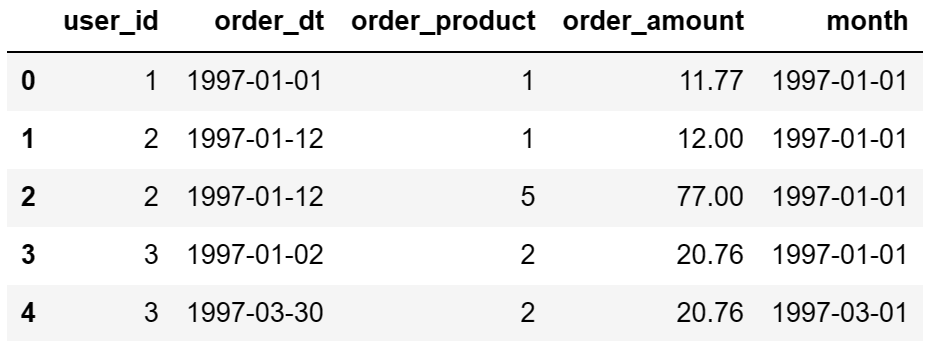
在源数据中添加一列表示月份:astype('datetime64[M]')

# 基于order_dt取出其中的月份
# astype('datetime64[M]')  将类型更换成 datetime64[M]，仅仅表示月份
df['order_dt'].astype('datetime64[M]')

0       1997-01-01
1       1997-01-01
2       1997-01-01
3       1997-01-01
4       1997-03-01
           ...    
69654   1997-04-01
69655   1997-04-01
69656   1997-03-01
69657   1997-03-01
69658   1997-03-01
Name: order_dt, Length: 69659, dtype: datetime64[ns]

df['month'] = df['order_dt'].astype('datetime64[M]')
df.head()

第二部分：按月数据分析

• 用户每月花费的总金额
  • 绘制曲线图展示
• 所有用户每月的产品购买量
• 所有用户每月的消费总次数
• 统计每月的消费人数

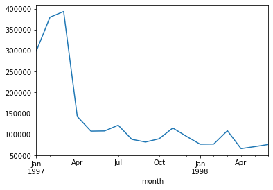
用户每月花费的总金额

df.groupby(by='month')['order_amount'].sum()

month
1997-01-01    299060.17
1997-02-01    379590.03
1997-03-01    393155.27
1997-04-01    142824.49
1997-05-01    107933.30
1997-06-01    108395.87
1997-07-01    122078.88
1997-08-01     88367.69
1997-09-01     81948.80
1997-10-01     89780.77
1997-11-01    115448.64
1997-12-01     95577.35
1998-01-01     76756.78
1998-02-01     77096.96
1998-03-01    108970.15
1998-04-01     66231.52
1998-05-01     70989.66
1998-06-01     76109.30
Name: order_amount, dtype: float64

绘制曲线图展示

# plt.plot(df.groupby(by='month')['order_amount'].sum())
df.groupby(by='month')['order_amount'].sum().plot()

AxesSubplot:xlabel='month'

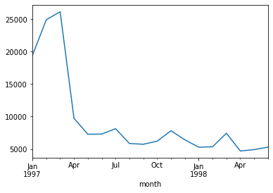
所有用户每月的产品购买量

df.groupby(by='month')['order_product'].sum().plot()

AxesSubplot:xlabel='month'

所有用户每月的消费总次数

• 原始数据中的一行数据表示一次消费记录

# count() 统计总共有多少行数据
df.groupby(by='month')['user_id'].count()

month
1997-01-01     8928
1997-02-01    11272
1997-03-01    11598
1997-04-01     3781
1997-05-01     2895
1997-06-01     3054
1997-07-01     2942
1997-08-01     2320
1997-09-01     2296
1997-10-01     2562
1997-11-01     2750
1997-12-01     2504
1998-01-01     2032
1998-02-01     2026
1998-03-01     2793
1998-04-01     1878
1998-05-01     1985
1998-06-01     2043
Name: user_id, dtype: int64

统计每月的消费人数

• 可能同一天一个用户会消费多次
• nunique表示统计去重后的个数

df.groupby(by='month')['user_id'].nunique()

month
1997-01-01    7846
1997-02-01    9633
1997-03-01    9524
1997-04-01    2822
1997-05-01    2214
1997-06-01    2339
1997-07-01    2180
1997-08-01    1772
1997-09-01    1739
1997-10-01    1839
1997-11-01    2028
1997-12-01    1864
1998-01-01    1537
1998-02-01    1551
1998-03-01    2060
1998-04-01    1437
1998-05-01    1488
1998-06-01    1506
Name: user_id, dtype: int64

第三部分：用户个体消费数据分析

• 用户消费总金额和消费总次数的统计描述
• 用户消费金额和消费产品数量的散点图
• 各个用户消费总金额的直方分布图(消费金额在1000之内的分布)
• 各个用户消费的总数量的直方分布图(消费商品的数量在100次之内的分布)

用户消费总金额和消费总次数的统计描述

每个用户消费的总金额

df.groupby(by='user_id')['order_amount'].sum()

user_id
1         11.77
2         89.00
3        156.46
4        100.50
5        385.61
          ...  
23566     36.00
23567     20.97
23568    121.70
23569     25.74
23570     94.08
Name: order_amount, Length: 23570, dtype: float64

每个用户消费的总次数

df.groupby(by='user_id').count()['order_dt']

user_id
1         1
2         2
3         6
4         4
5        11
         ..
23566     1
23567     1
23568     3
23569     1
23570     2
Name: order_dt, Length: 23570, dtype: int64

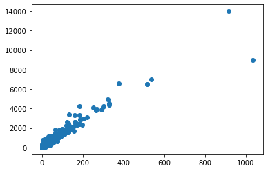
用户消费金额和消费产品数量的散点图

user_amount_sum = df.groupby(by='user_id')['order_amount'].sum()
user_product_sum = df.groupby(by='user_id')['order_product'].sum()
plt.scatter(user_product_sum,user_amount_sum)

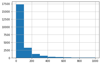
各个用户消费总金额的直方分布图(消费金额在1000之内的分布)

df.groupby(by='user_id').sum().query('order_amount <= 1000')['order_amount']
df.groupby(by='user_id').sum().query('order_amount <= 1000')['order_amount'].hist()

AxesSubplot:

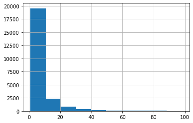
各个用户消费的总数量的直方分布图(消费商品的数量在100次之内的分布)

df.groupby(by='user_id').sum().query('order_product <= 100')['order_product'].hist()

AxesSubplot:

第四部分：用户消费行为分析（重点）

• 用户第一次消费的月份分布，和人数统计
  • 绘制线形图
• 用户最后一次消费的时间分布，和人数统计
  • 绘制线形图
• 新老客户的占比
  • 消费一次为新用户
  • 消费多次为老用户
    • 分析出每一个用户的第一次消费和最后一次消费的时间
      • agg(['func1','func2']):对分组后的结果进行多种指定聚合
    • 分析出新老客户的消费比例
• 用户分层
  • 分析得出每个用户的总购买量和总消费金额and最近一次消费的时间的表格RFM
  • RFM模型设计
    • R表示客户最近一次交易时间的间隔。
      • /np.timedelta64(1,'D')：去除days
    • F表示客户购买商品的总数量,F值越大，表示客户交易越频繁，反之则表示客户交易不够活跃。
    • M表示客户交易的金额。M值越大，表示客户价值越高，反之则表示客户价值越低。
    • 将R，F，M作用到RFM表中
  • 根据价值分层，将用户分为：
    • 重要价值客户
    • 重要保持客户
    • 重要挽留客户
    • 重要发展客户
    • 一般价值客户
    • 一般保持客户
    • 一般挽留客户
    • 一般发展客户
      • 使用已有的分层模型即可rfm_func

用户第一次消费的月份分布，和人数统计

第一次消费的月份

• 每一个用户消费月份的最小值就是该用户第一次消费的月份

df.groupby(by='user_id')['month'].min()

user_id
1       1997-01-01
2       1997-01-01
3       1997-01-01
4       1997-01-01
5       1997-01-01
           ...    
23566   1997-03-01
23567   1997-03-01
23568   1997-03-01
23569   1997-03-01
23570   1997-03-01
Name: month, Length: 23570, dtype: datetime64[ns]

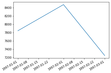
人数统计（绘制线形图）

# value_counts() 统计每一个元素出现的次数
df.groupby(by='user_id')['month'].min().value_counts()
df.groupby(by='user_id')['month'].min().value_counts().plot()

AxesSubplot:

用户最后一次消费的时间分布，和人数统计

• 用户消费月份的最大值就是用户最后一次消费的月份

最后一次消费的月份

df.groupby(by='user_id')['month'].max().value_counts()

1997-02-01    4912
1997-03-01    4478
1997-01-01    4192
1998-06-01    1506
1998-05-01    1042
1998-03-01     993
1998-04-01     769
1997-04-01     677
1997-12-01     620
1997-11-01     609
1998-02-01     550
1998-01-01     514
1997-06-01     499
1997-07-01     493
1997-05-01     480
1997-10-01     455
1997-09-01     397
1997-08-01     384
Name: month, dtype: int64

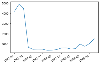
人数统计（绘制线形图）

df.groupby(by='user_id')['month'].max().value_counts().plot()

AxesSubplot:

新老客户的占比

• 消费一次为新用户，消费多次为老用户
• 如何获知用户是否为第一次消费？可以根据用户的消费时间进行判定？
  • 如果用户的第一次消费时间和最后一次消费时间一样，则该用户只消费了一次为新用户，否则为老用户

分析出每一个用户的第一次消费和最后一次消费的时间

new_old_user_df = df.groupby(by='user_id')['order_dt'].agg(['min','max'])  # agg对分组后的结果进行多种指定聚合
new_old_user_df

分析出新老客户的消费比例

new_old_user_df['min'] == new_old_user_df['max']  # True新用户，False老用户

user_id
1         True
2         True
3        False
4        False
5        False
         ...  
23566     True
23567     True
23568    False
23569     True
23570    False
Length: 23570, dtype: bool

# 统计True和False的个数
(new_old_user_df['min'] == new_old_user_df['max']).value_counts()

True     12054
False    11516
dtype: int64

用户分层

分析得出每个用户的总购买量和总消费金额and最近一次消费的时间的表格RFM

# 使用透视表
rfm = df.pivot_table(index='user_id',aggfunc={'order_product':'sum','order_amount':'sum','order_dt':"max"})
rfm

RFM模型设计

max_dt = df['order_dt'].max()  # 今天的日期

# 每个用户最后一次交易的时间
-(df.groupby(by='user_id')['order_dt'].max() - max_dt)

# R表示客户最近一次交易时间的间隔
# /np.timedelta64(1,'D')：去除days
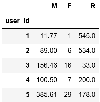
rfm['R'] = -(df.groupby(by='user_id')['order_dt'].max() - max_dt) /np.timedelta64(1,'D')

rfm.drop(labels='order_dt',axis=1,inplace=True)

# 重新给每一列取名
rfm.columns = ['M','F','R']
rfm.head()

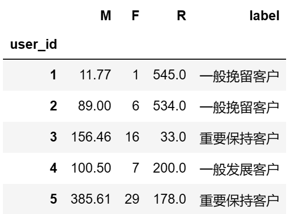
将用户根据价值分层

# 固定算法
def rfm_func(x):
    # 存储存储的是三个字符串形式的0或者1
    level = x.map(lambda x :'1' if x >= 0 else '0')
    label = level.R + level.F + level.M
    d = {
        '111':'重要价值客户',
        '011':'重要保持客户',
        '101':'重要挽留客户',
        '001':'重要发展客户',
        '110':'一般价值客户',
        '010':'一般保持客户',
        '100':'一般挽留客户',
        '000':'一般发展客户'
    }
    result = d[label]
    return result

# df.apply(func):可以对df中的行或者列进行某种（func）形式的运算
rfm['label'] = rfm.apply(lambda x : x - x.mean()).apply(rfm_func,axis = 1)
rfm.head()

第五部分：用户的生命周期（重点）

• 将用户划分为活跃用户和其他用户
  • 统计每个用户每个月的消费次数
  • 统计每个用户每个月是否消费，消费则记录为1,否则记录为0
    • 知识点：DataFrame的apply和applymap的区别
      • applymap:返回df
      • 将函数做用于DataFrame中的所有元素(elements)
      • apply:返回Series
      • apply()将一个函数作用于DataFrame中的每个行或者列
  • 将用户按照每一个月份分成：
    • unreg:观望用户（前两月没买，第三个月才第一次买,则用户前两个月为观望用户）
    • unactive:首月购买后，后序月份没有购买则在没有购买的月份中该用户的为非活跃用户
    • new:当前月就进行首次购买的用户在当前月为新用户
    • active:连续月份购买的用户在这些月中为活跃用户
    • return:购买之后间隔n月再次购买的第一个月份为该月份的回头客

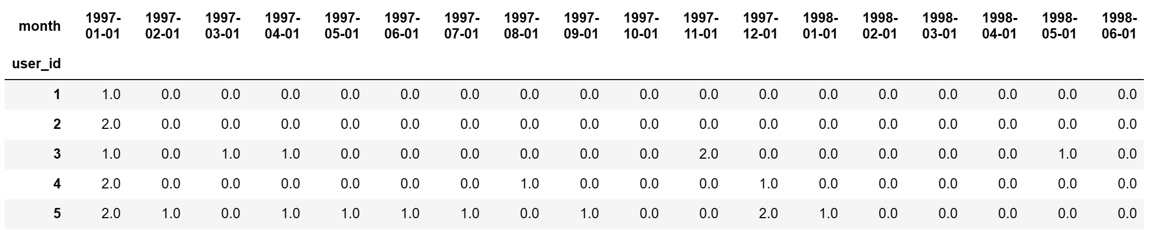
统计每个用户每个月的消费次数

user_month_count_df = df.pivot_table(index='user_id',values='order_dt',aggfunc='count',columns='month').fillna(0)
user_month_count_df.head()

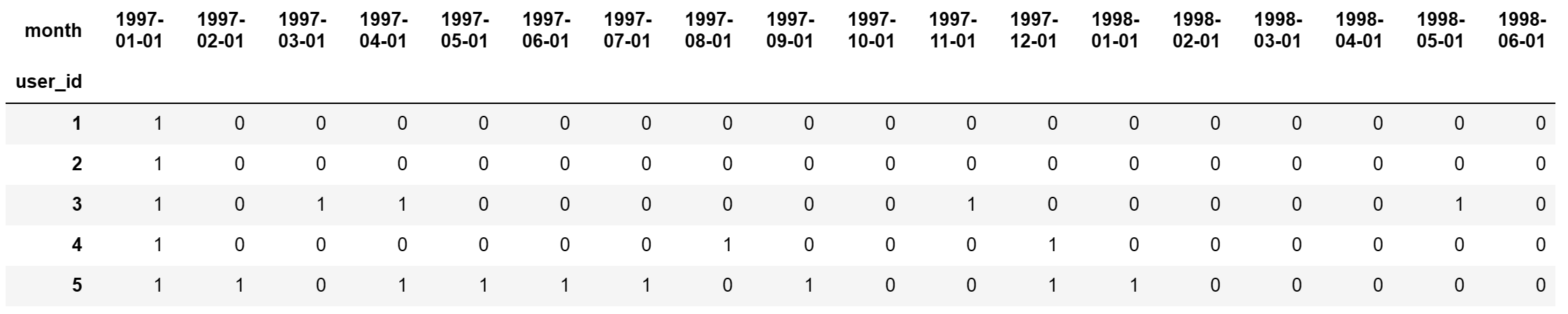
统计每个用户每个月是否消费，消费则记录为1,否则记录为0

# applymap() 对DataFrame中每个元素进行操作
# apply() 对DataFrame中行或列进行操作
df_purchase = user_month_count_df.applymap(lambda x:1 if x >= 1 else 0)
df_purchase.head()

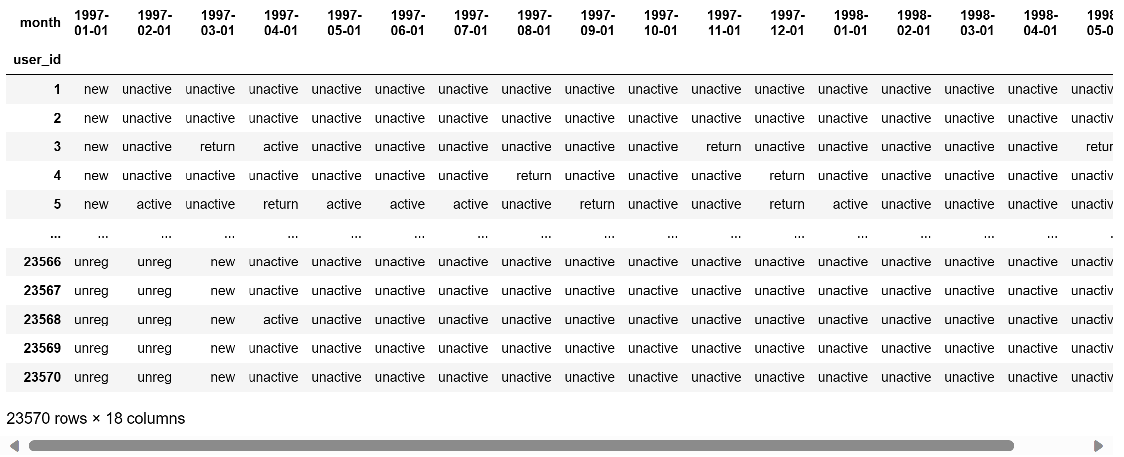
将用户按照每个月分成不同活跃度的用户

# 将df_purchase中的原始数据0和1修改为new，unactive......,返回新的df叫做df_purchase_new
# 固定算法
def active_status(data):
    status = []  # 某个用户每一个月的活跃度
    for i in range(18):        
        # 若本月没有消费
        if data[i] == 0:
            if len(status) > 0:
                if status[i-1] == 'unreg':
                    status.append('unreg')
                else:
                    status.append('unactive')
            else:
                status.append('unreg')
                    
        # 若本月消费
        else:
            if len(status) == 0:
                status.append('new')
            else:
                if status[i-1] == 'unactive':
                    status.append('return')
                elif status[i-1] == 'unreg':
                    status.append('new')
                else:
                    status.append('active')
    return status

pivoted_status = df_purchase.apply(active_status,axis = 1) 
pivoted_status.head()

user_id
1    [new, unactive, unactive, unactive, unactive, ...
2    [new, unactive, unactive, unactive, unactive, ...
3    [new, unactive, return, active, unactive, unac...
4    [new, unactive, unactive, unactive, unactive, ...
5    [new, active, unactive, return, active, active...
dtype: object

df_purchase_new = DataFrame(data=pivoted_status.values.tolist(),index=df_purchase.index,columns=df_purchase.columns)
df_purchase_new

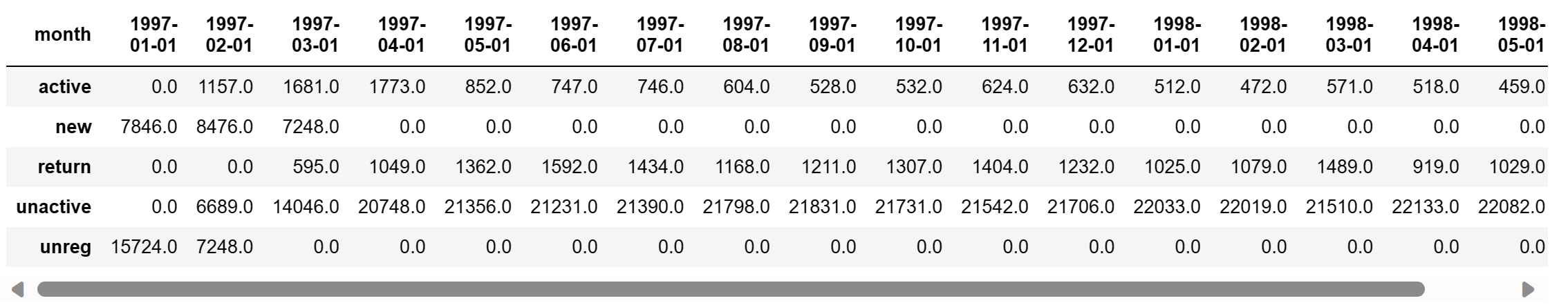
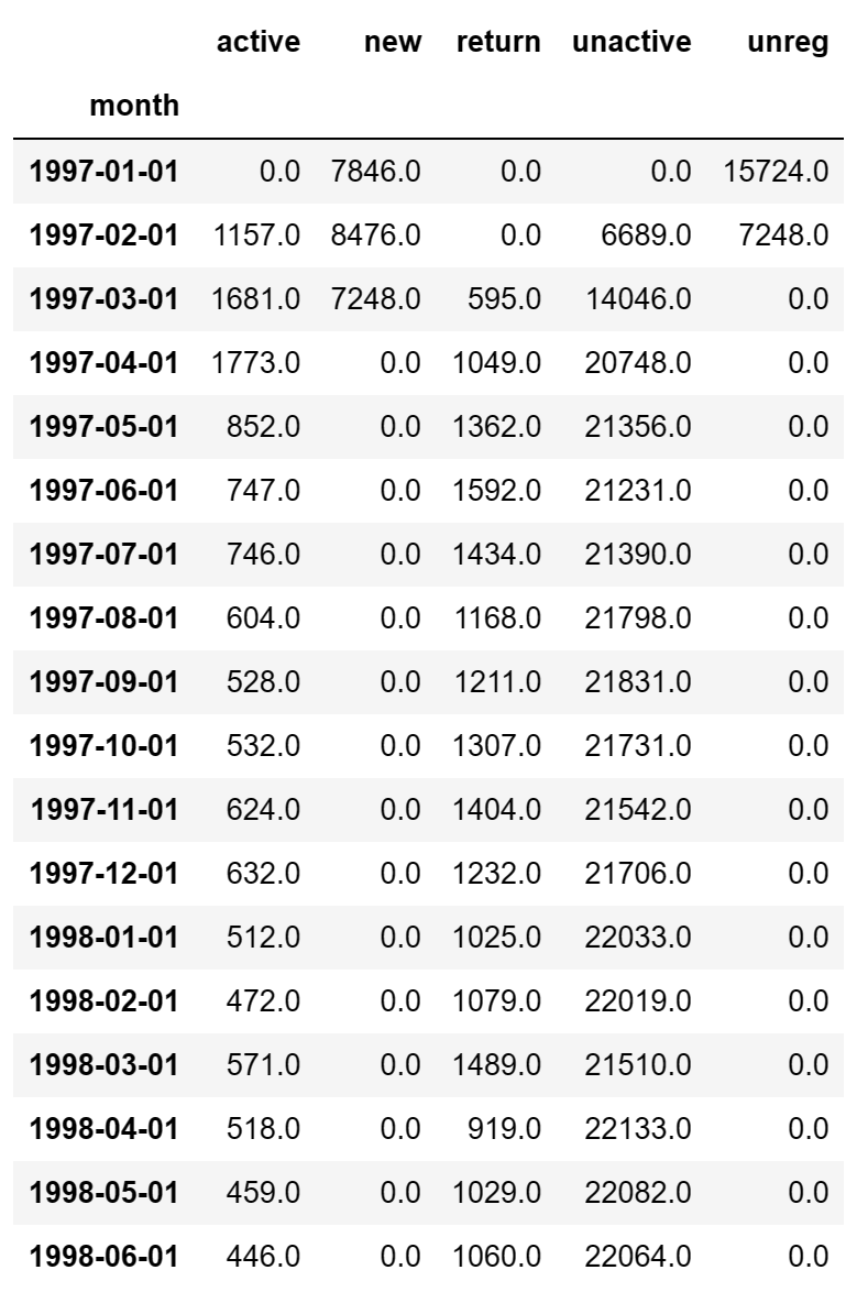
• 每月【不同活跃】用户的计数
  • purchase_status_ct = df_purchase_new.apply(lambda x : pd.value_counts(x)).fillna(0)
  • 转置进行最终结果的查看

purchase_status_ct = df_purchase_new.apply(lambda x : pd.value_counts(x)).fillna(0)
purchase_status_ct

purchase_status_ct.T