-
【单目3D目标检测】GUPNet论文精读与代码解析
Preface
Lu Y, Ma X, Yang L, et al. Geometry uncertainty projection network for monocular 3d object detection[C]. Proceedings of the IEEE/CVF International Conference on Computer Vision. 2021: 3111-3121.
Paper
CodeAbstract
在单目3D目标检测中,几何先验可以帮助深度推理,其中广泛使用的先验是透视投影模型。现有的投影模型方法通常是先估计2D和3D边界框的高度,然后通过投影公式 d e p t h = h 3 d ⋅ f / h 2 d depth =h_{3d}·f / h_{2d} depth=h3d⋅f/h2d ( f f f为摄像机焦距)推断出深度。由该公式推导出的深度与估计的2D/3D高度高度相关,因此高度估计的误差也会反映在估计的深度上。但是,高度估计的误差是不可避免的,特别是在3D高度估计不佳的情况下。因此,本文更关注由3D高度估计误差引起的深度推断误差。作者通过实验发现,3D高度的轻微偏差(0.1米)可能导致投影深度的显著偏移(甚至4米)。这种误差放大效应使得基于投影的方法的输出难以控制,显著影响了推理的可靠性和训练效率。因此,本文提出了一个包含几何不确定性投影(Geometry Uncertainty Projection,GUP)模块和分层任务学习(Hierarchical Task Learning,HTL)策略的几何不确定性投影网络来处理这些问题

Contributions
- 本文主要针对投影模型中的误差放大(Error Amplification)现象进行了两方面改进:
- GUP:3D高度估计质量的微小变化会引起深度估计质量的较大变化,这使得模型难以预测可靠的不确定性或置信度,导致输出不可控。为了解决这一问题,本文提出了GUP模块,根据分布形式而不是离散值来推断深度
- HTL:在训练阶段初期,2D/3D高度估计容易产生噪声,误差会被放大,导致深度估计过高。这样会误导网络的训练过程,导致最终性能的下降。为了解决训练的不稳定性,本文提出了HTL策略,目的是确保只有在所有的前置任务(如3D高度估计是深度估计的前置任务之一)都训练好了的情况下,才能训练每个任务
Pipeline
输入图像首先经过backbone(基于CenterNet)提取出2D的bounding box(输出一个2D heatmap、2D box的长宽和位置修正量),然后该bounding box经过ROI Align后提取出ROI特征,该特征会与3D坐标系进行concatenate从而获得最终的ROI特征,所有的3D信息推断均会在此ROI特征上进行。本文首先估计出3D box除了depth以外的所有参数。然后2D与3D bounding box的高度将被输入到GUP模块中提取出最终的depth,训练阶段HTL将会对每个部分进行控制从而实现multi-task learning

完整的Pipeline在
gupnet\code\lib\models\gupnet.py函数的GUPNet类中的__init__函数中定义Backbone
从代码中
config.yaml配置文件可以看到,GUPNet默认使用的Backbone为DLA34:model: type: 'gupnet' backbone: 'dla34' neck: 'DLAUp'- 1
- 2
- 3
- 4
我们可以在
gupnet\code\lib\models\gupnet.py函数的GUPNet类中的forward函数第一行加断点来进行debug,查看完整的Backbone信息: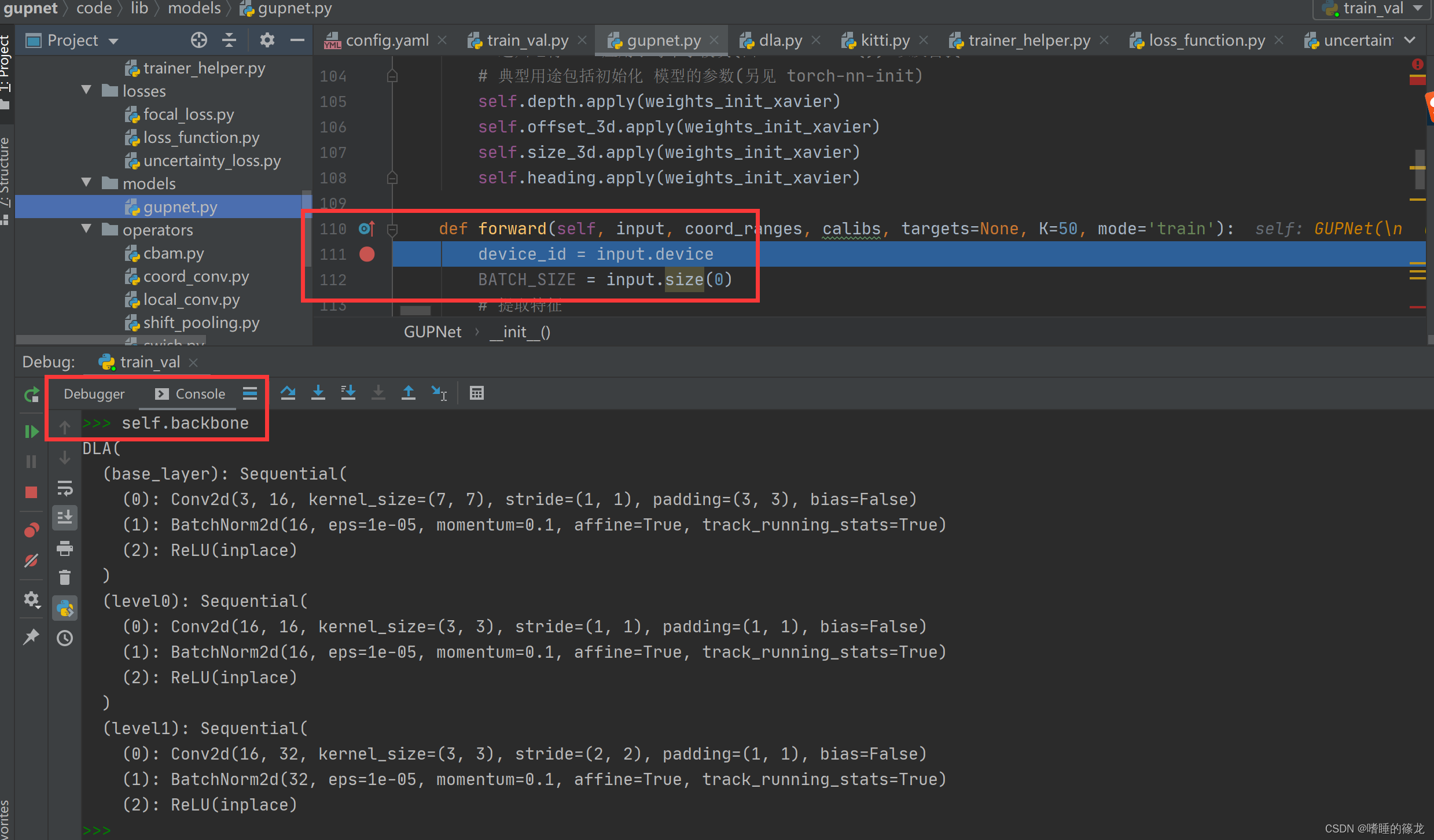
Backbone输出的6层feature map:Level Out-Channel Height Width 0 16 384 1280 1 32 192 640 2 64 96 320 3 128 48 160 4 256 24 80 5 512 12 40 Neck
同理,从
config.yaml配置文件可以看到,GUPNet默认使用的Neck为DLAUP:model: type: 'gupnet' backbone: 'dla34' neck: 'DLAUp'- 1
- 2
- 3
- 4
同样在debug中查看,注意这里的变量名为
self.feat_up: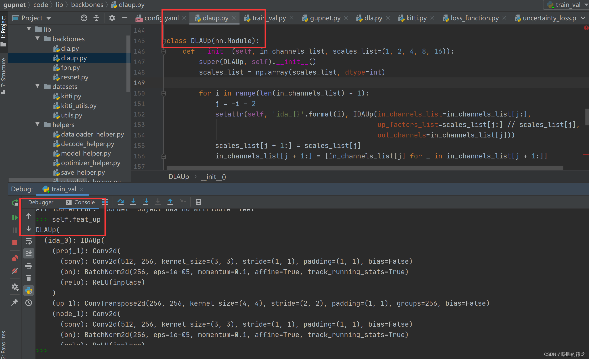
网络前向推断时,将Backbone输出的后4层feature map喂入Neck,最终输出最后一层feature map作为整个网络的输出:>> feat.shape >> torch.Size([B, 64, 96, 320])- 1
- 2
Head
gupnet\code\lib\models\gupnet.py函数的GUPNet类中的__init__函数定义了两大类Head:- 2D 检测输出,和CenterNet一样,包括三部分:
heatmap:所有类别的中心点(默认类别为3)offset_2d:2D框的偏移量size_2d: 2D框的宽高
- 这一部分直接在Neck输出的feature map上预测得到
# initialize the head of pipeline, according to heads setting. self.heatmap = nn.Sequential( nn.Conv2d(channels[self.first_level], self.head_conv, kernel_size=3, padding=1, bias=True), nn.ReLU(inplace=True), nn.Conv2d(self.head_conv, 3, kernel_size=1, stride=1, padding=0, bias=True)) self.offset_2d = nn.Sequential( nn.Conv2d(channels[self.first_level], self.head_conv, kernel_size=3, padding=1, bias=True), nn.ReLU(inplace=True), nn.Conv2d(self.head_conv, 2, kernel_size=1, stride=1, padding=0, bias=True)) self.size_2d = nn.Sequential( nn.Conv2d(channels[self.first_level], self.head_conv, kernel_size=3, padding=1, bias=True), nn.ReLU(inplace=True), nn.Conv2d(self.head_conv, 2, kernel_size=1, stride=1, padding=0, bias=True))- 1
- 2
- 3
- 4
- 5
- 6
- 7
- 8
- 9
- 10
- 11
- 12
- 13
- 3D 检测输出,包括四部分:
depth:输出2列信息,第一列为深度值,第二列为深度学习偏差(对数平方的形式)offset_3d:3D框在2D图像上的偏移量size_3d: 输出4列信息,前三列为3D框的长宽高,第四列为3D高度的偏差(对数平方的形式)heading:角度angle预测输出,将其划分为12份,分别预测12个类别分类输出(是哪一类),和12个回归预测输出(具体是多少)
- 这一部分不是直接在Neck输出的feature map上预测得到的,而是经过ROI Align后提取出ROI特征,该特征会再与3D
coord_ranges坐标系进行concatenate从而获得最终的ROI特征,所有的3D信息推断均会在此ROI特征上进行
self.depth = nn.Sequential( nn.Conv2d(channels[self.first_level] + 2 + self.cls_num, self.head_conv, kernel_size=3, padding=1, bias=True), nn.BatchNorm2d(self.head_conv), nn.ReLU(inplace=True), nn.AdaptiveAvgPool2d(1), nn.Conv2d(self.head_conv, 2, kernel_size=1, stride=1, padding=0, bias=True)) self.offset_3d = nn.Sequential( nn.Conv2d(channels[self.first_level] + 2 + self.cls_num, self.head_conv, kernel_size=3, padding=1, bias=True), nn.BatchNorm2d(self.head_conv), nn.ReLU(inplace=True), nn.AdaptiveAvgPool2d(1), nn.Conv2d(self.head_conv, 2, kernel_size=1, stride=1, padding=0, bias=True)) self.size_3d = nn.Sequential( nn.Conv2d(channels[self.first_level] + 2 + self.cls_num, self.head_conv, kernel_size=3, padding=1, bias=True), nn.BatchNorm2d(self.head_conv), nn.ReLU(inplace=True), nn.AdaptiveAvgPool2d(1), nn.Conv2d(self.head_conv, 4, kernel_size=1, stride=1, padding=0, bias=True)) self.heading = nn.Sequential( nn.Conv2d(channels[self.first_level] + 2 + self.cls_num, self.head_conv, kernel_size=3, padding=1, bias=True), nn.BatchNorm2d(self.head_conv), nn.ReLU(inplace=True), nn.AdaptiveAvgPool2d(1), nn.Conv2d(self.head_conv, 24, kernel_size=1, stride=1, padding=0, bias=True))- 1
- 2
- 3
- 4
- 5
- 6
- 7
- 8
- 9
- 10
- 11
- 12
- 13
- 14
- 15
- 16
- 17
- 18
- 19
- 20
- 21
- 22
- 23
- 24
Loss
各个head的损失函数如下:
heatmap:Focal Lossoffset2s:L1 Losssize2d:L1 Losssize3d:长和宽为L1 Loss,占2/3,3D 高为laplacian_aleatoric_uncertainty_loss(),占1/3offset3d:L1 Lossdepth:laplacian_aleatoric_uncertainty_loss()heading:cls为CE,reg为L1 Loss
GUP
In Paper
由于误差放大效应的存在,使得获取高质量得分变得非常困难。其本质就是因为投影过程对于uncertainty regression部分而言是不可知(agnostic)的,其没有直接参与到投影过程的计算中,因此使得不确定度的估计质量不高。为了实现对depth进行更好的uncertainty的估计,本文认为把投影过程体现在uncertainty的计算过程中尤为重要。因此本文采用基于概率模型的方法对uncertainty的估计同样引入投影先验

-
首先假设投影过程中的 h 3 d h_{3d} h3d 是拉普拉斯分布 L a ( μ h , λ h ) La(\mu_h,\lambda_h) La(μh,λh) ,也即 X ∼ L a ( μ , λ ) , f X ( x ) = 1 2 λ exp ( − ∣ x − μ ∣ λ ) X \sim L a(\mu, \lambda), f_X(x)=\frac{1}{2 \lambda} \exp \left(-\frac{|x-\mu|}{\lambda}\right) X∼La(μ,λ),fX(x)=2λ1exp(−λ∣x−μ∣),此时 h 3 d h_{3d} h3d的损失函数可定义为:
L h 3 d = 2 σ h ∣ μ h − h 3 d g t ∣ + log ( σ h ) \mathcal{L}_{h_{3d}}=\frac{\sqrt{2}}{\sigma_h}\left|\mu_h-h_{3d}^{g t}\right|+\log \left(\sigma_h\right) Lh3d=σh2∣∣μh−h3dgt∣∣+log(σh) -
将其代入投影模型,可计算出depth为:
d p = f ⋅ h 3 d h 2 d = f ⋅ ( λ h ⋅ X + μ h ) h 2 d = f ⋅ λ h h 2 d ⋅ X + f ⋅ μ h h 2 d dp=f⋅h3dh2d=f⋅(λh⋅X+μh)h2d=f⋅λhh2d⋅X+f⋅μhh2ddp=h2df⋅h3d=h2df⋅(λh⋅X+μh)=h2df⋅λh⋅X+h2df⋅μh
其中 X X X是一个归一化的拉普拉斯分布 L a ( 0 , 1 ) La(0,1) La(0,1)。可以看到深度估计值 d p d_p dp的期望 μ p \mu_p μp和标准差 σ p \sigma_p σp分别为 f ⋅ μ h h 2 d \frac{f · \mu_h}{h_{2d}} h2df⋅μh和 f ⋅ σ h h 2 d \frac{f · \sigma_h}{h_{2d}} h2df⋅σh,其中 σ h \sigma_h σh是拉普拉斯分布 L a ( μ h , λ h ) La(\mu_h,\lambda_h) La(μh,λh)对应的标准差( σ h 2 = 2 λ h 2 \sigma_h^2=2\lambda_h^2 σh2=2λh2 ) -
对于结果 d p d_p dp而言,均值 μ p \mu_p μp对应投影depth结果,而 σ p \sigma_p σp则反应了投影不确定度。在此基础上,为了更精准的depth输出,本文额外让神经网络预测出一个depth的修正值(depth bias),本文假设该修正值也是拉普拉斯分布 L a ( μ b , λ b ) La(\mu_b,\lambda_b) La(μb,λb),因此最终depth则变成:
d = L a ( μ p , σ p ) + L a ( μ b , σ b ) μ d = μ p + μ b , σ d = ( σ p ) 2 + ( σ b ) 2 . d=La(μp,σp)+La(μb,σb)μd=μp+μb,σd=√(σp)2+(σb)2.d=La(μp,σp)+La(μb,σb)μd=μp+μb,σd=(σp)2+(σb)2.
那么这时输出端的不确定度就同时反应了投影模型放大的输入端的不确定性以及网络bias引入的不确定度,称为基于几何的不确定度(Geometry based Uncertainty,GeU) -
为了优化最终深度分布,本文应用了不确定性回归损失:
L depth = 2 σ d ∣ μ d − d g t ∣ + log ( σ d ) \mathcal{L}_{\text {depth }}=\frac{\sqrt{2}}{\sigma_d}\left|\mu_d-d^{g t}\right|+\log \left(\sigma_d\right) Ldepth =σd2∣∣μd−dgt∣∣+log(σd)
为了简化起见,假定深度分布属于拉普拉斯分布。整体损失会使投影结果更接近GT,梯度同时影响深度偏差、 h 2 d h_{2d} h2d和 h 3 d h_{3d} h3d。此外,在优化过程中还训练了三维高度和深度偏差的不确定性 -
为了获得最终得分,本文进一步将深度的不确定性 σ d \sigma_d σd将其映射为0 ~ 1之间的值,通过指数函数表示深度的不确定性-置信度(Uncertainty-Confidence,UnC):
p d e p t h = exp ( − σ d ) p_{depth}=\exp \left(-\sigma_d\right) pdepth=exp(−σd)
它可以为每个投影深度提供更精确的置信度 -
最终的推理得分可以计算为:
p 3 d = p 3 d ∣ 2 d ⋅ p 2 d = p depth ⋅ p 2 d p_{3 d}=p_{3 d \mid 2 d} \cdot p_{2 d}=p_{\text {depth }} \cdot p_{2 d} p3d=p3d∣2d⋅p2d=pdepth ⋅p2d
该评分既代表了二维检测置信度,也代表了深度推理置信度,可以指导更好的可靠性。其计算过程引入了投影模型的先验,因此由投影模型引起的误差放大效应可以被一定程度上解决,因为由 h 3 d h_{3d} h3d估计误差引起的放大误差会被很好的反应在计算的不确定度中,所以基于此不确定度得到的得分质量将大幅上升
In Code
在代码中,GUP模块主要对应两部分:
- 前向传播计算深度值
- 对应代码:
gupnet\code\lib\models\gupnet.py函数中GUPNet类的get_roi_feat_by_mask函数
# compute heights of projected objects box2d_height = torch.clamp(box2d_masked[:, 4] - box2d_masked[:, 2], min=1.0) # compute real 3d height # [B * 4] size3d_offset = self.size_3d(roi_feature_masked)[:, :, 0, 0] # [B * 1], 最后一列预测3D 高度的偏差, 实际为log(σ_b^2),即对数方差形式 h3d_log_std = size3d_offset[:, 3:4] size3d_offset = size3d_offset[:, :3] # 3D的宽高预测值 size_3d = (self.mean_size[cls_ids[mask].long()] + size3d_offset) # depth = f * (h_3d / h_2d) 投影转换公式 depth_geo = size_3d[:, 0] / box2d_height.squeeze() * roi_calibs[:, 0, 0] # 网络预测的depth 其shape: torch.Size([:, 2]) # 第一列:深度值depth # 第二列:depth的修正值(depth bias), 实际为log(σ_b^2),即对数方差形式 depth_net_out = self.depth(roi_feature_masked)[:, :, 0, 0] # d_p的方差σ_p^2 depth_geo_log_std = ( h3d_log_std.squeeze() + 2 * (roi_calibs[:, 0, 0].log() - box2d_height.log())).unsqueeze(-1) # 最终的depth的方差: log(σ_d^2) = log(σ_p^2 + σ_b^2) depth_net_log_std = torch.logsumexp(torch.cat([depth_net_out[:, 1:2], depth_geo_log_std], -1), -1, keepdim=True) # depth_net_out[:, 0:1].sigmoid() 归一化 (0, 1) # 最终输出的depth包括两列: # - 第一列为depth的预测值, 由 网络预测输出 + 投影公式转换 得到 # - 第二列为depth的修正值, 实际为log(σ_b^2),即对数方差形式 depth_net_out = torch.cat( [(1. / (depth_net_out[:, 0:1].sigmoid() + 1e-6) - 1.) + depth_geo.unsqueeze(-1), depth_net_log_std], -1) res['train_tag'] = torch.ones(num_masked_bin).type(torch.bool).to(device_id) res['heading'] = self.heading(roi_feature_masked)[:, :, 0, 0] res['depth'] = depth_net_out res['offset_3d'] = self.offset_3d(roi_feature_masked)[:, :, 0, 0] res['size_3d'] = size3d_offset res['h3d_log_variance'] = h3d_log_std- 1
- 2
- 3
- 4
- 5
- 6
- 7
- 8
- 9
- 10
- 11
- 12
- 13
- 14
- 15
- 16
- 17
- 18
- 19
- 20
- 21
- 22
- 23
- 24
- 25
- 26
- 27
- 28
- 29
- 30
- 31
- 32
- 33
- 34
- 35
- 反向传播计算深度值的loss
- 对应代码:
gupnet\code\lib\losses\uncertainty_loss.py中的laplacian_aleatoric_uncertainty_loss函数
# 拉普拉斯任意不确定损失 def laplacian_aleatoric_uncertainty_loss(input, target, log_variance, reduction='mean'): assert reduction in ['mean', 'sum'] loss = 1.4142 * torch.exp(-0.5*log_variance) * torch.abs(input - target) + 0.5*log_variance return loss.mean() if reduction == 'mean' else loss.sum()- 1
- 2
- 3
- 4
- 5
input<=> μ d \mu_d μdtarget<=> d g t d^{gt} dgtlog_variance<=> 2 l o g ( σ d ) 2log(\sigma_d) 2log(σd)
计算过程如下:- 原计算公式: L depth = 2 σ d ∣ μ d − d g t ∣ + log ( σ d ) \mathcal{L}_{\text {depth }}=\frac{\sqrt{2}}{\sigma_d}\left|\mu_d-d^{g t}\right|+\log \left(\sigma_d\right) Ldepth =σd2∣μd−dgt∣+log(σd)
- 令: v = l o g ( σ d 2 ) = 2 l o g ( σ d ) v=log(\sigma_d^2)=2log(\sigma_d) v=log(σd2)=2log(σd)
- 则代码中的计算公式为:
L
depth
=
2
e
x
p
(
−
0.5
v
)
∣
μ
d
−
d
g
t
∣
+
0.5
v
\mathcal{L}_{\text {depth }}=\sqrt{2}exp(-0.5v)|\mu_d-d^{gt}|+0.5v
Ldepth =2exp(−0.5v)∣μd−dgt∣+0.5v
HTL
In Paper
这一部分在论文中的思路是:先给出最终的结论,即最终我的损失函数是什么样的,然后一步一步地解释这里面每一项是什么来的,以及具体的含义,相当于一种倒序结构
GUP模块主要解决推理阶段的误差放大效应。然而,这种效应也破坏了训练过程。具体来说,在训练开始时,对 h 2 d h_{2d} h2d和 h 3 d h_{3d} h3d的预测都很不准确,这将误导整个训练,损害性能。为了解决这个问题,本文设计了一个分层任务学习(HTL)来控制每个阶段每个任务的权重,最终总的损失函数 L total \mathcal{L}_{\text {total }} Ltotal 如下所示:
L total = ∑ i ∈ T w i ( t ) ⋅ L i \mathcal{L}_{\text {total }}=\sum_{i \in \mathcal{T}} w_i(t) \cdot \mathcal{L}_i Ltotal =i∈T∑wi(t)⋅Li
其中各参数含义如下:- T \mathcal{T} T:总的任务集合
- t t t:当前第几个epoch
- L i \mathcal{L}_i Li:第 i i i个任务的损失函数
- w i ( t ) w_i(t) wi(t):第 i i i个任务在第 t t t个epoch阶段的损失函数的权重
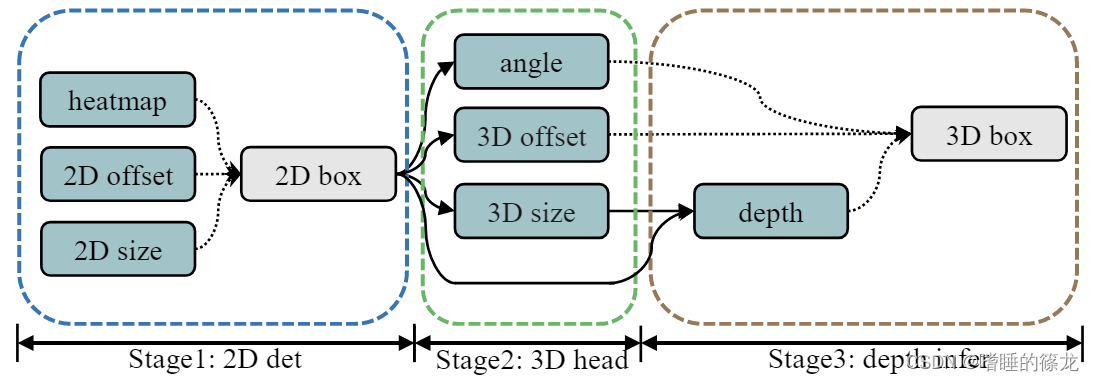
首先,本文认为每个任务(task)都应该在它的前任务(pre-task)训练好之后才开始训练,并且将任务划分为不同的阶段,如下图所示。第一阶段是2D检测,包括heatmap、2D 偏移量、2D尺寸。第二阶段是3D head,包含角度、3D偏移量和3D尺寸的3D头。这些3D任务都是建立在ROI特征之上的,所以2D检测阶段的任务是它们的前置任务。同样,最后一个阶段是深度推断,它的前置任务是3D尺寸和2D检测阶段的所有任务,因为深度预测依赖于2D高度和2D高度
所以总得来说,我们需要两个元素实现这件事情:1). 任务学习状态评估:用于评估先制任务的学习状态,2). 当前任务控制器:当先制任务学习达标后,提高当前任务的权重:
- 为了对每个任务进行充分的训练,目标是随着训练的进行将
w
i
(
t
)
w_i(t)
wi(t)从0逐渐增加到1。因此采用多项式时间调度函数作为加权函数:
w i ( t ) = ( t T ) 1 − α i ( t ) , α i ( t ) ∈ [ 0 , 1 ] w_i(t)=\left(\frac{t}{T}\right)^{1-\alpha_i(t)}, \quad \alpha_i(t) \in[0,1] wi(t)=(Tt)1−αi(t),αi(t)∈[0,1]
其中, T T T为训练总epoch数,归一化时间变量 t T \frac{t}{T} Tt可以自动调整时间刻度。 α i ( t ) \alpha_i(t) αi(t)是第 t t t个epoch的调整参数,对应第 i i i个任务的所有前置任务。 α i \alpha_i αi越大, w i w_i wi增加越快,即如果所有的前置任务都得到了很好的训练,那么 α i \alpha_i αi就应该很大,否则就应该很小

-
α
i
(
⋅
)
\alpha_i(·)
αi(⋅)与其所有前置任务有关,将所有前置任务的学习情况指标相乘表示为该任务的损失函数权重:
α i ( t ) = ∏ j ∈ P i l s j ( t ) \alpha_i(t)=\prod_{j \in \mathcal{P}_i} l s_j(t) αi(t)=j∈Pi∏lsj(t)
其中, P i \mathcal{P}_i Pi表示第 i i i个任务的所有前置任务集合, l s j ls_j lsj表示这些前置任务中,第 j j j个任务的学习情况指标(越好,值越大,取值介于0 ~ 1之间)。这个公式意味着 α i \alpha_i αi只有在所有前置任务都达到高 l s j ls_j lsj(训练良好)时才会得到较高的值 - 这里作者使用尺度不变因子(Scale-Invariant Factor)来表示每个任务的学习情况:
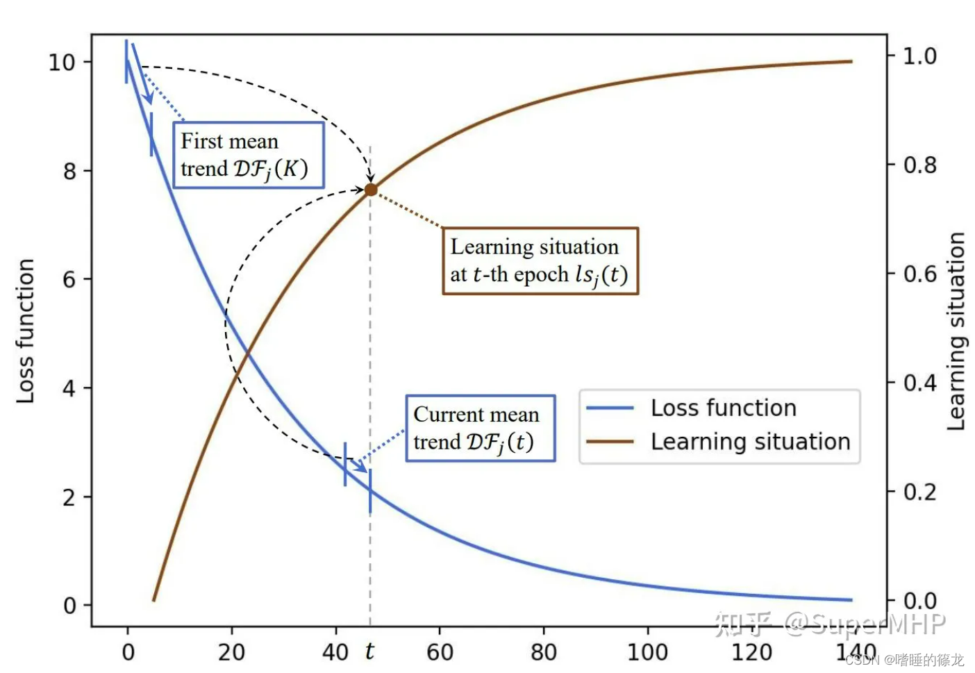
l s j ( t ) = D F j ( K ) − D F j ( t ) D F j ( K ) D F j ( t ) = 1 K ∑ t ^ = t − K t − 1 ∣ L j ′ ( t ^ ) ∣ lsj(t)=DFj(K)−DFj(t)DFj(K)DFj(t)=1Kt−1∑ˆt=t−K|L′j(ˆt)|lsj(t)DFj(t)=DFj(K)DFj(K)−DFj(t)=K1t^=t−K∑t−1∣∣Lj′(t^)∣∣
其中, L j ′ ( t ^ ) \mathcal{L}_j^{\prime}(\hat{t}) Lj′(t^)为 L j ( ) \mathcal{L}_j() Lj()在第 t ^ \hat t t^个epoch时的一阶导数,可以表示损失函数的局部变化趋势。 D F j ( t ) \mathcal{D} \mathcal{F}_j(t) DFj(t)计算第 t t t个epoch之前的最近 K K K个epoch导数的平均值,用来反映平均值的变化趋势。 D F j ( K ) \mathcal{D} \mathcal{F}_j(K) DFj(K)表示第 j j j个任务训练开始时的前 K K K个epoch的变化趋势。如果 L j \mathcal{L}_j Lj在最近的 K K K个epoch内快速下降, D F j \mathcal{D} \mathcal{F}_j DFj将得到较大的值。因此 l s j ls_j lsj公式表示比较当前训练的变化趋势与刚开始训练时变化趋势之间的差异。如果当前的损失趋势与开始的趋势相似,则指标会给出一个很小的值,这意味着该任务没有很好地训练。反之,如果任务趋于收敛,则lj值将趋近于1,表示该任务的学习情况是很好地,具体图解如下所示:
在总体设计的基础上,每个项的损失权重可以动态地反映其前置任务的学习情况,使训练更加稳定
In Code
- 对应代码:
gupnet\code\lib\losses\loss_function.py中的Hierarchical_Task_Learning函数 - 这一部分在代码中的逻辑如下:
- 首先初始化7个Loss的权重:2D相关的都为1,3D相关的都为0
- 前5个epoch不做任何处理,权重值不变
- 5个epoch之后,开始计算当前epoch的局部变化趋势(往前数5个epoch内),并且保存前5个epoch内的变化趋势不变
- 根据论文中的公式更新权重,直到训练结束
# HTL:Hierarchical Task Learning 分层任务学习 # 2D 损失函数的权重一直不变,都为1 # 3D 损失函数的权重初始化为0,在第5个epoch之后,开始变化 # 具体变化规则取决于之前任务的学习情况 # 任务的学习情况则是通过损失函数的局部变化趋势来判断 class Hierarchical_Task_Learning: def __init__(self, epoch0_loss, stat_epoch_nums=5): self.index2term = [*epoch0_loss.keys()] self.term2index = {term: self.index2term.index(term) for term in self.index2term} # term2index # self.term2index: { # 'seg_loss': 0, 'offset2d_loss': 1, 'size2d_loss': 2, # 'depth_loss': 3, 'offset3d_loss': 4, 'size3d_loss': 5, 'heading_loss': 6} self.stat_epoch_nums = stat_epoch_nums # 对应论文中的K,即与前K个epoch的loss进行比较 self.past_losses = [] self.loss_graph = {'seg_loss': [], 'size2d_loss': [], 'offset2d_loss': [], 'offset3d_loss': ['size2d_loss', 'offset2d_loss'], 'size3d_loss': ['size2d_loss', 'offset2d_loss'], 'heading_loss': ['size2d_loss', 'offset2d_loss'], 'depth_loss': ['size2d_loss', 'size3d_loss', 'offset2d_loss']} def compute_weight(self, current_loss, epoch): T = 140 # compute initial weights loss_weights = {} ''' current_loss_0:{ 'seg_loss': tensor(75.1708, device='cuda:0'), 'offset2d_loss': tensor(1.0958, device='cuda:0'), 'size2d_loss': tensor(19.7375, device='cuda:0'), 'depth_loss': tensor(8.5812, device='cuda:0'), 'offset3d_loss': tensor(0.9910, device='cuda:0'), 'size3d_loss': tensor(0.9233, device='cuda:0'), 'heading_loss': tensor(3.7395, device='cuda:0')} eval_loss_input: tensor([[75.1708, 1.0958, 19.7375, 8.5812, 0.9910, 0.9233, 3.7395]], device='cuda:0') ''' eval_loss_input = torch.cat([_.unsqueeze(0) for _ in current_loss.values()]).unsqueeze(0) for term in self.loss_graph: if len(self.loss_graph[term]) == 0: loss_weights[term] = torch.tensor(1.0).to(current_loss[term].device) else: loss_weights[term] = torch.tensor(0.0).to(current_loss[term].device) # update losses list if len(self.past_losses) == self.stat_epoch_nums: past_loss = torch.cat(self.past_losses) # 5个list -> [5, 7]的tensor # 使用差分计算5个epoch内,loss的变化趋势,一阶导数 mean_diff = (past_loss[:-2] - past_loss[2:]).mean(0) # 以下代码只运行一次,即保存前5个epoch的loss变化趋势 if not hasattr(self, 'init_diff'): self.init_diff = mean_diff # 表示该epoch下loss的变化趋势 c_weights = 1 - (mean_diff / self.init_diff).relu().unsqueeze(0) print('c_weights: ', c_weights) print('mean_diff: ', mean_diff) print('self.init_diff: ', self.init_diff) # t / T time_value = min(((epoch - 5) / (T - 5)), 1.0) for current_topic in self.loss_graph: # 只有3D 预测信息的loss会变化,2D的不会变('size2d_loss','size3d_loss','offset2d_loss') if len(self.loss_graph[current_topic]) != 0: control_weight = 1.0 for pre_topic in self.loss_graph[current_topic]: # 该epoch下的调整参数 control_weight *= c_weights[0][self.term2index[pre_topic]] # (t / T)^(1 - α) loss_weights[current_topic] = time_value ** (1 - control_weight) # pop first list 丢掉第一个epoch的loss self.past_losses.pop(0) # 添加当前epoch的loss self.past_losses.append(eval_loss_input) return loss_weights def update_e0(self, eval_loss): self.epoch0_loss = torch.cat([_.unsqueeze(0) for _ in eval_loss.values()]).unsqueeze(0)- 1
- 2
- 3
- 4
- 5
- 6
- 7
- 8
- 9
- 10
- 11
- 12
- 13
- 14
- 15
- 16
- 17
- 18
- 19
- 20
- 21
- 22
- 23
- 24
- 25
- 26
- 27
- 28
- 29
- 30
- 31
- 32
- 33
- 34
- 35
- 36
- 37
- 38
- 39
- 40
- 41
- 42
- 43
- 44
- 45
- 46
- 47
- 48
- 49
- 50
- 51
- 52
- 53
- 54
- 55
- 56
- 57
- 58
- 59
- 60
- 61
- 62
- 63
- 64
- 65
- 66
- 67
- 68
- 69
- 70
- 71
- 72
- 73
- 74
- 75
- 76
- 77
- 78
Refernece
-
相关阅读:
docker安装redis
wordpress搭建自己的博客详细过程以及踩坑
基于STM32单片机的温湿度检测报警器(数码管)(Proteus仿真+程序)
详解动态规划
多测师肖sir_高级金牌讲师_jenkins搭建
【C++】友元类 ( 友元类简介 | 友元类声明 | 友元类单向性 | 友元类继承性 | 友元类作用 | 友元类和友元函数由来 | Java 反射机制 | C / C++ 编译过程 )
Ylearn因果推断入门实践——Kaggle银行客户流失
内存管理---分页机制
Docker容器网络安全性最佳实践:防止容器间攻击
自动化测试:webdriver的断言详解
- 原文地址:https://blog.csdn.net/weixin_43799388/article/details/127689177
