-
Pytorch实战:基于鲸鱼WOA优化1DCNN的轴承故障诊断
目录
0.引言
采用1DCNN进行轴承故障诊断建模,并基于鲸鱼优化算法WOA对1DCNN的超参数进行优化,以实现更高的精度。建立一个两层的1DCNN,优化的参数包括学习率、训练次数、batchsize,卷积层1的核数量、核大小,池化层1的核大小,卷积层2的核数量、核大小,池化层2的核大小,全连接层1、全连接层2的节点数,总共11个超参数。
1.关键点
在Pytorch中,卷积层与池化层由于无法像tensorflow中一样,将padding设置成“same”模式,因此每一层的输出要手动计算,并且与全连接层的输入节点参数也要精确计算出来,否则节点数不匹配,容易报错。而我们采用优化算法来进行优化的,每一层的参数不是固定的,所以第一步是实现像tensorflow中一样,将卷积层与池化层设计成padding具备“same”模式的结构,代码如下:
- class Conv1d(torch.nn.Module):
- def __init__(self, in_channels, out_channels, kernel_size, bias=True, padding_layer=nn.ReflectionPad1d):
- super().__init__()
- ka = kernel_size // 2
- kb = ka - 1 if kernel_size % 2 == 0 else ka
- self.net = torch.nn.Sequential(
- padding_layer((ka,kb)),
- nn.Conv1d(in_channels, out_channels, kernel_size, bias=bias)
- )
- def forward(self, x):
- return self.net(x)
- class MaxPool1d(torch.nn.Module):
- def __init__(self, kernel_size):
- super().__init__()
- self.net=torch.nn.MaxPool1d(kernel_size=kernel_size)
- def forward(self, x):
- x1=self.net(x)
- padsize=x.size(2)-x1.size(2)
- ka = padsize // 2
- kb = ka if padsize % 2 == 0 else ka+1
- return F.pad(x1,(ka,kb))
- net1=Conv1d(1,3,10)#输入通道、输出通道数、卷积核大小
- net2=MaxPool1d(3)#池化核大小
- dummy=torch.rand(16,1,101)
- print(net1(dummy).size())
- print(net1(dummy).size())
- # torch.Size([16, 3, 101])
- # torch.Size([16, 3, 101])
可以看出,无论怎么设置输入的长度,与卷积、池化参数,他的输出长度都是与输入的长度都是一样的。
采用上述代码设计一个两层的1DCNN,代码如下
- class ConvNet(torch.nn.Module):
- def __init__(self,num_input,nk1,k1,pk1,nk2,k2,pk2,fc1,fc2, num_classes):
- super(ConvNet, self).__init__()
- # 1D-CNN 输入1*1024振动信号
- self.net = nn.Sequential(
- Conv1d(1,nk1 , kernel_size=k1),
- MaxPool1d(kernel_size=pk1),
- nn.ReLU(),
- nn.BatchNorm1d(nk1),
- Conv1d(nk1, nk2, kernel_size=k2),
- MaxPool1d(kernel_size=pk2),
- nn.ReLU(),
- nn.BatchNorm1d(nk2)
- )
- self.feature_extractor = nn.Sequential(
- nn.Linear(num_input*nk2, fc1),
- nn.ReLU(),
- # nn.Dropout(0.5),
- nn.Linear(fc1, fc2))
- self.classifier=nn.Sequential(
- nn.ReLU(),
- nn.Linear(fc2, num_classes),
- )
- def forward(self,x):
- x= self.net(x)#进行卷积+池化操作提取振动信号特征
- x=x.view(-1, x.size(1)*x.size(2))
- feature = self.feature_extractor(x)#将上述特征拉伸为向量输入进全连接层实现分类
- logits = self.classifier(feature)#将上述特征拉伸为向量输入进全连接层实现分类
- probas = F.softmax(logits, dim=1)# softmax分类器
- return logits,probas
- net=ConvNet(101,8,3,3,16,3,4,128,128,10)
- dummy=torch.rand(16,1,101)
- print(net(dummy)[0].size())
- # torch.Size([16, 10])
- net=ConvNet(111,8,7,3,16,7,4,256,128,10)
- dummy=torch.rand(16,1,111)
- print(net(dummy)[0].size())
- # torch.Size([16, 10])
可以看出,无论怎么设置输入的长度,与卷积、池化参数,他的输出都是16x10(16是batchsize,10是类别数)
2.WOA优化1DCNN超参数实战
2.1 数据准备
数据依旧采用48k的驱动端轴承故障诊断数据,每种故障样本数为200,每个样本的长度为1024,按照7:2:1的比例划分训练集、验证集、测试集
- #coding:utf-8
- from scipy.io import loadmat
- from scipy.io import savemat
- import numpy as np
- import os
- from sklearn import preprocessing # 0-1编码
- from sklearn.model_selection import StratifiedShuffleSplit # 随机划分,保证每一类比例相同
- def prepro(d_path, length=864, number=1000, normal=True, rate=[0.7, 0.2, 0.1], enc=True, enc_step=28):
- """对数据进行预处理,返回train_X, train_Y, valid_X, valid_Y, test_X, test_Y样本.
- :param d_path: 源数据地址
- :param length: 信号长度,默认2个信号周期,864
- :param number: 每种信号个数,总共10类,默认每个类别1000个数据
- :param normal: 是否标准化.True,Fales.默认True
- :param rate: 训练集/验证集/测试集比例.默认[0.5,0.25,0.25],相加要等于1
- :param enc: 训练集、验证集是否采用数据增强.Bool,默认True
- :param enc_step: 增强数据集采样顺延间隔
- :return: Train_X, Train_Y, Valid_X, Valid_Y, Test_X, Test_Y
- ```
- import preprocess.preprocess_nonoise as pre
- train_X, train_Y, valid_X, valid_Y, test_X, test_Y = pre.prepro(d_path=path,
- length=864,
- number=1000,
- normal=False,
- rate=[0.5, 0.25, 0.25],
- enc=True,
- enc_step=28)
- ```
- """
- # 获得该文件夹下所有.mat文件名
- filenames = os.listdir(d_path)
- def capture(original_path):
- """读取mat文件,返回字典
- :param original_path: 读取路径
- :return: 数据字典
- """
- files = {}
- for i in filenames:
- # 文件路径
- file_path = os.path.join(d_path, i)
- file = loadmat(file_path)
- file_keys = file.keys()
- for key in file_keys:
- if 'DE' in key:
- files[i] = file[key].ravel()
- return files
- def slice_enc(data, slice_rate=rate[1] + rate[2]):
- """将数据切分为前面多少比例,后面多少比例.
- :param data: 单挑数据
- :param slice_rate: 验证集以及测试集所占的比例
- :return: 切分好的数据
- """
- keys = data.keys()
- Train_Samples = {}
- Test_Samples = {}
- for i in keys:
- slice_data = data[i]
- all_lenght = len(slice_data)
- end_index = int(all_lenght * (1 - slice_rate))
- samp_train = int(number * (1 - slice_rate)) # 700
- Train_sample = []
- Test_Sample = []
- if enc:
- enc_time = length // enc_step
- samp_step = 0 # 用来计数Train采样次数
- for j in range(samp_train):
- random_start = np.random.randint(low=0, high=(end_index - 2 * length))
- label = 0
- for h in range(enc_time):
- samp_step += 1
- random_start += enc_step
- sample = slice_data[random_start: random_start + length]
- Train_sample.append(sample)
- if samp_step == samp_train:
- label = 1
- break
- if label:
- break
- else:
- for j in range(samp_train):
- random_start = np.random.randint(low=0, high=(end_index - length))
- sample = slice_data[random_start:random_start + length]
- Train_sample.append(sample)
- # 抓取测试数据
- for h in range(number - samp_train):
- random_start = np.random.randint(low=end_index, high=(all_lenght - length))
- sample = slice_data[random_start:random_start + length]
- Test_Sample.append(sample)
- Train_Samples[i] = Train_sample
- Test_Samples[i] = Test_Sample
- return Train_Samples, Test_Samples
- # 仅抽样完成,打标签
- def add_labels(train_test):
- X = []
- Y = []
- label = 0
- for i in filenames:
- x = train_test[i]
- X += x
- lenx = len(x)
- Y += [label] * lenx
- label += 1
- return X, Y
- # one-hot编码
- def one_hot(Train_Y, Test_Y):
- Train_Y = np.array(Train_Y).reshape([-1, 1])
- Test_Y = np.array(Test_Y).reshape([-1, 1])
- Encoder = preprocessing.OneHotEncoder()
- Encoder.fit(Train_Y)
- Train_Y = Encoder.transform(Train_Y).toarray()
- Test_Y = Encoder.transform(Test_Y).toarray()
- Train_Y = np.asarray(Train_Y, dtype=np.int32)
- Test_Y = np.asarray(Test_Y, dtype=np.int32)
- return Train_Y, Test_Y
- def scalar_stand(Train_X, Test_X):
- # 用训练集标准差标准化训练集以及测试集
- scalar = preprocessing.StandardScaler().fit(Train_X)
- Train_X = scalar.transform(Train_X)
- Test_X = scalar.transform(Test_X)
- return Train_X, Test_X
- def valid_test_slice(Test_X, Test_Y):
- test_size = rate[2] / (rate[1] + rate[2])
- ss = StratifiedShuffleSplit(n_splits=1, test_size=test_size)
- for train_index, test_index in ss.split(Test_X, Test_Y):
- X_valid, X_test = Test_X[train_index], Test_X[test_index]
- Y_valid, Y_test = Test_Y[train_index], Test_Y[test_index]
- return X_valid, Y_valid, X_test, Y_test
- # 从所有.mat文件中读取出数据的字典
- data = capture(original_path=d_path)
- # 将数据切分为训练集、测试集
- train, test = slice_enc(data)
- # 为训练集制作标签,返回X,Y
- Train_X, Train_Y = add_labels(train)
- # 为测试集制作标签,返回X,Y
- Test_X, Test_Y = add_labels(test)
- # 为训练集Y/测试集One-hot标签
- Train_Y, Test_Y = one_hot(Train_Y, Test_Y)
- # 训练数据/测试数据 是否标准化.
- if normal:
- Train_X, Test_X = scalar_stand(Train_X, Test_X)
- else:
- # 需要做一个数据转换,转换成np格式.
- Train_X = np.asarray(Train_X)
- Test_X = np.asarray(Test_X)
- # 将测试集切分为验证集合和测试集.
- Valid_X, Valid_Y, Test_X, Test_Y = valid_test_slice(Test_X, Test_Y)
- return Train_X, Train_Y, Valid_X, Valid_Y, Test_X, Test_Y
- if __name__ == "__main__":
- path = '0HP/'
- train_X, train_Y, valid_X, valid_Y, test_X, test_Y = prepro(d_path=path,
- length=1024,
- number=200,
- normal=True,
- rate=[0.7, 0.2, 0.1],
- enc=False,
- enc_step=28)
- savemat("data_process.mat", {'train_X': train_X,'train_Y': train_Y,
- 'valid_X': valid_X,'valid_Y': valid_Y,
- 'test_X': test_X,'test_Y': test_Y})
2.2 1DCNN故障诊断建模
基于1中的1DCNN进行故障诊断建模,参数我们随意设置,测试集精度为80.5%(可以手动调参,提高精度,不过我比较懒,而且要对比出优化的重要性)
- # coding: utf-8
- # In[1]: 导入必要的库函数
- import numpy as np
- import torch
- import torch.nn as nn
- import torch.nn.functional as F
- from sklearn.preprocessing import MinMaxScaler,StandardScaler
- from model import ConvNet,Model_fit
- import matplotlib.pyplot as plt
- if torch.cuda.is_available():
- torch.backends.cudnn.deterministic = True
- from scipy.io import loadmat
- device = torch.device("cuda:0" if torch.cuda.is_available() else "cpu")
- # In[2] 加载数据
- num_classes=10
- # 振动信号----1D-CNN输入
- data=loadmat('data_process.mat')
- x_train1=data['train_X']
- x_valid1=data['valid_X']
- y_train=data['train_Y'].argmax(axis=1)
- y_valid=data['valid_Y'].argmax(axis=1)
- ss1=StandardScaler().fit(x_train1) #MinMaxScaler StandardScaler
- x_train1=ss1.transform(x_train1)
- x_valid1=ss1.transform(x_valid1)
- x_train1=x_train1.reshape(-1,1,1024)
- x_valid1=x_valid1.reshape(-1,1,1024)
- # 转换为torch的输入格式
- train_features1 = torch.tensor(x_train1).type(torch.FloatTensor)
- valid_features1 = torch.tensor(x_valid1).type(torch.FloatTensor)
- train_labels = torch.tensor(y_train).type(torch.LongTensor)
- valid_labels = torch.tensor(y_valid).type(torch.LongTensor)
- print(train_features1.shape)
- print(train_labels.shape)
- N=train_features1.size(0)
- # In[3]: 参数设置
- learning_rate = 0.005#学习率
- num_epochs = 10#迭代次数
- batch_size = 64 #batchsize
- # In[4]: 模型设置
- torch.manual_seed(0)
- torch.cuda.manual_seed(0)
- model=ConvNet(train_features1.size(-1),8,3,3,16,3,4,128,128,10)
- train_again=True # True就重新训练
- if train_again:
- # In[5]:
- Model=Model_fit(model,batch_size,learning_rate,num_epochs,device,verbose=True)
- Model.train(train_features1,train_labels,valid_features1,valid_labels)
- model= Model.model
- train_loss=Model.train_loss
- valid_loss=Model.valid_loss
- valid_acc=Model.valid_acc
- train_acc=Model.train_acc
- torch.save(model,'model/W_CNN1.pkl')#保存整个网络参数
- # In[]
- #loss曲线
- plt.figure()
- plt.plot(np.array(train_loss),label='train')
- plt.plot(np.array(valid_loss),label='valid')
- plt.title('loss curve')
- plt.legend()
- plt.savefig('图片保存/loss')
- # accuracy 曲线
- plt.figure()
- plt.plot(np.array(train_acc),label='train')
- plt.plot(np.array(valid_acc),label='valid')
- plt.title('accuracy curve')
- plt.legend()
- plt.savefig('图片保存/accuracy')
- plt.show()
- else:
- model=torch.load('model/W_CNN1.pkl',map_location=torch.device('cpu'))#加载模型
- Model=Model_fit(model,batch_size,learning_rate,num_epochs,device,verbose=True)
- # In[6]: 利用训练好的模型 对测试集进行分类
- #提取测试集
- x_test1=data['test_X']
- y_test=data['test_Y'].argmax(axis=1)
- x_test1=ss1.transform(x_test1)
- x_test1=x_test1.reshape(-1,1,1024)
- test_features1 = torch.tensor(x_test1).type(torch.FloatTensor)
- test_labels = torch.tensor(y_test).type(torch.LongTensor)
- _,teac=Model.compute_accuracy(test_features1,test_labels)
- print('CNN直接分类的测试集正确率为:',teac*100,'%')
2.3 采用WOA优化1DCNN超参数
以最小化验证集分类错误率为适应度函数进行网络优化,目的是找到一组最优超参数,使得训练好的网络的验证集分类错误率最低。
- # coding: utf-8
- # In[1]: 导入必要的库函数
- import numpy as np
- import torch
- import torch.nn as nn
- import torch.nn.functional as F
- from sklearn.preprocessing import MinMaxScaler,StandardScaler
- from model import ConvNet,Model_fit
- from optim import WOA,HUATU
- import matplotlib.pyplot as plt
- if torch.cuda.is_available():
- torch.backends.cudnn.deterministic = True
- from scipy.io import loadmat
- device = torch.device("cuda:0" if torch.cuda.is_available() else "cpu")
- #torch.manual_seed(0)
- # In[2] 加载数据
- num_classes=10
- # 振动信号----1D-CNN输入
- data=loadmat('data_process.mat')
- x_train1=data['train_X']
- x_valid1=data['valid_X']
- y_train=data['train_Y'].argmax(axis=1)
- y_valid=data['valid_Y'].argmax(axis=1)
- ss1=StandardScaler().fit(x_train1) #MinMaxScaler StandardScaler
- x_train1=ss1.transform(x_train1)
- x_valid1=ss1.transform(x_valid1)
- x_train1=x_train1.reshape(-1,1,1024)
- x_valid1=x_valid1.reshape(-1,1,1024)
- # 转换为torch的输入格式
- train_features1 = torch.tensor(x_train1).type(torch.FloatTensor)
- valid_features1 = torch.tensor(x_valid1).type(torch.FloatTensor)
- train_labels = torch.tensor(y_train).type(torch.LongTensor)
- valid_labels = torch.tensor(y_valid).type(torch.LongTensor)
- # In[] WOA优化CNN
- optim_again = True # 为 False 的时候就直接加载之间优化好的超参建建
- # 训练模型
- if optim_again:
- best,trace,process=WOA(train_features1,train_labels,valid_features1,valid_labels)
- trace,process=np.array(trace),np.array(process)
- np.savez('model/woa_result.npz',trace=trace,best=best,process=process)
- else:
- para=np.load('model/woa_result.npz')
- trace=para['trace'].reshape(-1,)
- process=para['process']
- best=para['best'].reshape(-1,)
- HUATU(trace)
- # In[3]: 参数设置
- pop=best
- learning_rate = pop[0] # 学习率
- num_epochs = int(pop[1]) # 迭代次数
- batch_size = int(pop[2]) # batchsize
- nk1 = int(pop[3]) # conv1核数量
- k1 = int(pop[4]) # conv1核大小
- pk1 = int(pop[5]) # pool1核大小
- nk2 = int(pop[6]) # conv2核数量
- k2 = int(pop[7]) # conv2核大小
- pk2 = int(pop[8]) # pool2核大小
- fc1 = int(pop[9]) #全连接层1节点数
- fc2 = int(pop[10]) #全连接层2节点数
- torch.manual_seed(0)
- torch.cuda.manual_seed(0)
- model=ConvNet(train_features1.size(-1),nk1,k1,pk1,nk2,k2,pk2,fc1,fc2,10)
- train_again= True #True 就重新训练
- # In[5]:
- if train_again:
- Model=Model_fit(model,batch_size,learning_rate,num_epochs,device,verbose=True)
- Model.train(train_features1,train_labels,valid_features1,valid_labels)
- model= Model.model
- train_loss=Model.train_loss
- valid_loss=Model.valid_loss
- valid_acc=Model.valid_acc
- train_acc=Model.train_acc
- torch.save(model,'model/W_CNN2.pkl')#保存整个网络参数
- #loss曲线
- plt.figure()
- plt.plot(np.array(train_loss),label='train')
- plt.plot(np.array(valid_loss),label='valid')
- plt.title('loss curve')
- plt.legend()
- plt.savefig('图片保存/loss')
- # accuracy 曲线
- plt.figure()
- plt.plot(np.array(train_acc),label='train')
- plt.plot(np.array(valid_acc),label='valid')
- plt.title('accuracy curve')
- plt.legend()
- plt.savefig('图片保存/accuracy')
- plt.show()
- else:
- model=torch.load('model/W_CNN2.pkl',map_location=torch.device('cpu'))#加载模型
- Model=Model_fit(model,batch_size,learning_rate,num_epochs,device,verbose=True)
- # In[6]: 利用训练好的模型 对测试集进行分类
- #提取测试集
- x_test1=data['test_X']
- y_test=data['test_Y'].argmax(axis=1)
- x_test1=ss1.transform(x_test1)
- x_test1=x_test1.reshape(-1,1,1024)
- test_features1 = torch.tensor(x_test1).type(torch.FloatTensor)
- test_labels = torch.tensor(y_test).type(torch.LongTensor)
- _,teac=Model.compute_accuracy(test_features1,test_labels)
- print('WOA-CNN分类的测试集正确率为:',teac*100,'%')
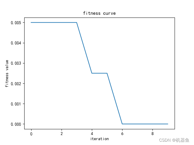
由于是最小化 验证集分类错误率为适应度函数,所以适应度曲线是一条下降的曲线。
3.代码
代码链接见评论区我的评论
-
相关阅读:
dp记录。
R-FCN: Object Detection via Region-based Fully Convolutional Networks
Web3 新手攻略:9 个不可或缺的 APP 助力你踏入加密领域
【Java】Java中对List进行排序
excel文件双击 该文件没有与之关联的应用来执行操作
微软校园大使喊你来秋招啦!
流程图渲染方式:Canvas vs SVG
相机平行状态下模型无法初始化到桌面
华为机试 - 水仙花数 Ⅰ
C++初阶--内存管理
- 原文地址:https://blog.csdn.net/qq_41043389/article/details/127799188
