-
【毕业设计】基于大数据的京东消费行为分析与可视化 - python 机器学习
1 前言
🔥 这两年开始毕业设计和毕业答辩的要求和难度不断提升,传统的毕设题目缺少创新和亮点,往往达不到毕业答辩的要求,这两年不断有学弟学妹告诉学长自己做的项目系统达不到老师的要求。
为了大家能够顺利以及最少的精力通过毕设,学长分享优质毕业设计项目,今天要分享的是
🚩 基于大数据的京东消费行为分析与可视化
🥇学长这里给一个题目综合评分(每项满分5分)
- 难度系数:3分
- 工作量:3分
- 创新点:3分
🧿 选题指导, 项目分享:
2 数据处理
import pandas as pd import numpy as np import matplotlib.pyplot as plt import seaborn as sns import warnings import seaborn as sns from pylab import * from pyecharts.charts import * from pyecharts import options as opts from pyecharts.commons.utils import JsCode import textwrap # 中文设置 plt.rcParams['font.sans-serif']=['Microsoft YaHei'] plt.rcParams['axes.unicode_minus']=False plt.rc('font',family = 'Microsoft YaHei',size = '15') warnings.filterwarnings("ignore") %matplotlib inline- 1
- 2
- 3
- 4
- 5
- 6
- 7
- 8
- 9
- 10
- 11
- 12
- 13
- 14
- 15
- 16
- 17
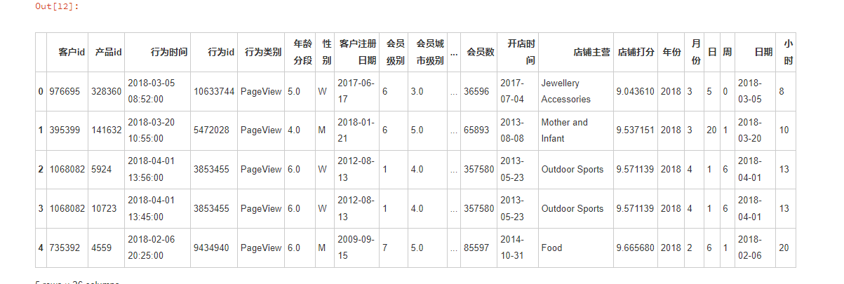
# 读取数据 data = pd.read_excel('D:/data/京东消费者分析数据.xlsx') data.head(10)- 1
- 2
- 3
# 查看数据量 print('数据条数:{} \n数据字段:{}'.format(data.shape[0],data.shape[1]))- 1
- 2
#字段中文命名 data.columns = ["客户id","产品id","行为时间","行为id","行为类别","年龄分段","性别","客户注册日期",\ "会员级别","会员城市级别","产品品牌","店铺id","产品类别","产品上市日期","商家id",\ "粉丝数","会员数","开店时间","店铺主营","店铺打分"] data.head(10)- 1
- 2
- 3
- 4
- 5

data.info()- 1
# 缺失率 data.isnull().mean()- 1
- 2
缺失字段只有“年龄分段”,“会员城市级别”,“开店时间”。
其中“年龄分段”,“会员城市级别”数据量占比很少,可以去除
“开店时间”缺失达到1/3,暂时保留数据,需要相关分析时再去除。# 删除缺失值 data.dropna(subset=['年龄分段','会员城市级别'],inplace=True) print(data.shape) data.isnull().mean()- 1
- 2
- 3
- 4
# 删除重复值 data.drop_duplicates(inplace=True) print(data.shape)- 1
- 2
- 3
- 4
# 数据描述 print('行为类别包含:{}'.format(data['行为类别'].unique())) print('性别包含:{}'.format(data['性别'].unique())) print('产品类别包含:{}'.format(data["产品类别"].unique())) print('年龄分段包含:{}'.format(data['年龄分段'].unique())) data[['年龄分段','粉丝数','会员数','店铺打分']].describe()[1:]- 1
- 2
- 3
- 4
- 5
- 6
- 7
# 异常值判断 print(len(data[data['店铺打分'] < 0])) print(len(data[data['店铺打分'] < 0]) / data.shape[0])- 1
- 2
- 3
- 4
店铺打分出现负值,考虑到可能是差评,但是常规评分为(0-10),认为0分已经是差评了,具体要看实际业务评定,这里考虑到数量极少,可以视为0分处理
#替换异常值 data['店铺打分'] = data['店铺打分'].apply(lambda x: 0 if x<0 else x) data[['年龄分段','粉丝数','会员数','店铺打分']].describe()[1:]- 1
- 2
- 3
# 转化行为时间,提取年份、月份、日、周数据 pd.to_datetime(data['行为时间'],format="%Y-%m-%d") data['年份'] = data['行为时间'].dt.year data['月份'] = data['行为时间'].dt.month data['日'] = data['行为时间'].dt.day data['周'] = data['行为时间'].dt.weekday data['日期'] = data['行为时间'].dt.date data['小时'] = data['行为时间'].dt.hour # 重建data索引 data = data.reset_index(drop = True) data.head()- 1
- 2
- 3
- 4
- 5
- 6
- 7
- 8
- 9
- 10
- 11
3 数据分析
每日UV(访客数)与每日PV(访客量)
# 计算每日的UV uv_data = data.drop_duplicates(subset = ['日期','客户id']) uv_data = uv_data[['日期','客户id']].groupby(['日期']).count().reset_index() uv_data.rename(columns = {'客户id':'日UV'},inplace = True) uv_data.head()- 1
- 2
- 3
- 4
- 5
# 绘制平滑好看的折线图函数 def echarts_line(x,y,title = '主标题',subtitle = '副标题',label = '图例'): """ x: 函数传入x轴标签数据 y:函数传入y轴数据 title:主标题 subtitle:副标题 label:图例 """ line = Line( init_opts=opts.InitOpts( bg_color='#080b30', # 设置背景颜色 theme='dark', # 设置主题 width='1200px', # 设置图的宽度 height='600px', # 设置图的高度 ) ) line.add_xaxis(x) line.add_yaxis( label, y, is_symbol_show=False, # 是否显示数据标签点 is_smooth=True, # 设置曲线平滑 label_opts=opts.LabelOpts( is_show=False, # 是否显示数据 ), itemstyle_opts=opts.ItemStyleOpts(color='#00ca95'), # 设置系列颜色 # 线条粗细阴影设置 linestyle_opts={ "normal": { "color": "#00ca95", #线条颜色 "shadowColor": 'rgba(0, 0, 0, .3)', #阴影颜色和不透明度 "shadowBlur": 2, #阴影虚化大小 "shadowOffsetY": 5, #阴影y偏移量 "shadowOffsetX": 5, #阴影x偏移量 "width": 6 # 线条粗细 }, }, # 阴影设置 areastyle_opts={ "normal": { "color": JsCode("""new echarts.graphic.LinearGradient(0, 0, 0, 1, [{ offset: 0, color: 'rgba(0,202,149,0.5)' }, { offset: 1, color: 'rgba(0,202,149,0)' } ], false)"""), #设置底色色块渐变 "shadowColor": 'rgba(0,202,149, 0.9)', #设置底色阴影 "shadowBlur": 20 #设置底色阴影大小 } }, ) line.set_global_opts( # 标题设置 title_opts=opts.TitleOpts( title=title, # 主标题 subtitle=subtitle, # 副标题 pos_left='center', # 标题展示位置 title_textstyle_opts=dict(color='#fff') # 设置标题字体颜色 ), # 图例设置 legend_opts=opts.LegendOpts( is_show=True, # 是否显示图例 pos_left='right', # 图例显示位置 pos_top='3%', #图例距离顶部的距离 orient='horizontal' # 图例水平布局 ), tooltip_opts=opts.TooltipOpts( is_show=True, # 是否使用提示框 trigger='axis', # 触发类型 is_show_content = True, trigger_on='mousemove|click', # 触发条件,点击或者悬停均可出发 axis_pointer_type='cross', # 指示器类型,鼠标移动到图表区可以查看效果 # formatter = '{a}
{b}:{c}人' # 文本内容 ), datazoom_opts=opts.DataZoomOpts( range_start=0, # 开始范围 range_end=50, # 结束范围 # orient='vertical', # 设置为垂直布局 type_='slider', # slider形式 is_zoom_lock=False, # 锁定区域大小 # pos_left='1%' # 设置位置 ), yaxis_opts=opts.AxisOpts( is_show=True, splitline_opts=opts.SplitLineOpts(is_show=False), # 分割线 axistick_opts=opts.AxisTickOpts(is_show=False), # 刻度不显示 ), # 关闭Y轴显示 xaxis_opts=opts.AxisOpts( boundary_gap=False, # 两边不显示间隔 axistick_opts=opts.AxisTickOpts(is_show=True), # 刻度不显示 splitline_opts=opts.SplitLineOpts(is_show=False), # 分割线不显示 axisline_opts=opts.AxisLineOpts(is_show=True), # 轴不显示 axislabel_opts=opts.LabelOpts( # 坐标轴标签配置 font_size=10, # 字体大小 font_weight='light' # 字重 ) ), ) return line.render_notebook()- 1
- 2
- 3
- 4
- 5
- 6
- 7
- 8
- 9
- 10
- 11
- 12
- 13
- 14
- 15
- 16
- 17
- 18
- 19
- 20
- 21
- 22
- 23
- 24
- 25
- 26
- 27
- 28
- 29
- 30
- 31
- 32
- 33
- 34
- 35
- 36
- 37
- 38
- 39
- 40
- 41
- 42
- 43
- 44
- 45
- 46
- 47
- 48
- 49
- 50
- 51
- 52
- 53
- 54
- 55
- 56
- 57
- 58
- 59
- 60
- 61
- 62
- 63
- 64
- 65
- 66
- 67
- 68
- 69
- 70
- 71
- 72
- 73
- 74
- 75
- 76
- 77
- 78
- 79
- 80
- 81
- 82
- 83
- 84
- 85
- 86
- 87
- 88
- 89
- 90
- 91
- 92
- 93
- 94
- 95
- 96
- 97
- 98
- 99
- 100
- 101
- 102
- 103
# 日UV变化图 echarts_line(uv_data['日期'].tolist(),uv_data['日UV'].tolist(),title = '日UV变化图',subtitle = '每日UV变化图',label = 'UV')- 1
- 2

因为月份过少,且4月数据不完整,只分析每日UV(访客数)。
1.在2月上旬属于平台高峰期,且在2月15日出现了最低谷,大概率是京东平台在2月上旬为2月14日情人节准备了预热活动,加上客户为情人节准备礼物的原因。
2.3月27日,3月28两日的UV出现了异常,出现断崖式低峰,而3月29日又立刻恢复了正常,需要重点查明UV低下的原因,暂时分析的原因可能是数据出错或者两日内平台出现技术上的问题,使得用户无法登录。
3.其他日期的数据变化相对较为平缓,属于正常趋势。
# 日PV变化 day_pv_data = data[['日期','客户id']].groupby('日期').count().reset_index() day_pv_data.rename(columns = {'客户id':'日PV'},inplace = True) day_pv_data.head()- 1
- 2
- 3
- 4
# 日pv变化图 echarts_line(day_pv_data['日期'].tolist(),day_pv_data['日PV'].tolist(),title = '日PV变化图',subtitle = '每日PV变化图',label = 'PV')- 1
- 2

日PV(访客量)的变化趋势跟日UV(访客数)的访客变化趋势大致一致,分析一致,不多累述。
人群图像
# 客户性别比例 user_gender = data[['客户id','性别']].drop_duplicates(subset = ['客户id']) gender_rate = user_gender.groupby('性别').count().reset_index() gender_rate.rename(columns={'客户id':'人数'},inplace=True) gender_rate.drop(gender_rate[gender_rate['性别']=='U'].index, inplace=True) gender_rate['比例'] = gender_rate["人数"] / gender_rate["人数"].sum() gender_rate = gender_rate.reset_index(drop=True) gender_rate- 1
- 2
- 3
- 4
- 5
- 6
- 7
- 8
# 购买数量性别比例 buy_gender = data[['产品id','性别']] gender_buy_rate = buy_gender.groupby('性别').count().reset_index() gender_buy_rate.rename(columns={'产品id':'购买数量'},inplace=True) gender_buy_rate.drop(gender_buy_rate[gender_buy_rate['性别']=='U'].index, inplace=True) gender_buy_rate['比例'] = gender_buy_rate["购买数量"] / gender_buy_rate["购买数量"].sum() gender_buy_rate = gender_buy_rate.reset_index(drop=True) gender_buy_rate- 1
- 2
- 3
- 4
- 5
- 6
- 7
- 8
# 年龄分布 age_data = data[['客户id','年龄分段']].drop_duplicates(subset = ['客户id']) age_rate = age_data.groupby('年龄分段').count().reset_index() age_rate.drop(age_rate[age_rate['年龄分段']==3].index,inplace=True) age_rate.rename(columns={'客户id':'人数'},inplace=True) age_rate['比例'] = age_rate['人数'] / age_rate['人数'].sum() age_rate- 1
- 2
- 3
- 4
- 5
- 6
- 7
- 8
c = ( Pie() .add( "", [list(z) for z in zip(age_rate['年龄分段'].tolist(),age_rate['比例'].round(4).tolist())], center=["35%", "50%"], ) .set_global_opts( title_opts=opts.TitleOpts(title="年龄分布比例"), legend_opts=opts.LegendOpts(pos_left="15%"), ) .set_series_opts(label_opts=opts.LabelOpts(formatter="{b}: {c}")) ) c.render_notebook()- 1
- 2
- 3
- 4
- 5
- 6
- 7
- 8
- 9
- 10
- 11
- 12
- 13
- 14

性别分布上,该平台无论客户人数还是购买产品数量上的男女比例都是男性占大多数,约比女性多一倍,产品和营销活动可以多以男性为主,但是考虑到部分产品品牌类别原因,如珠宝,化妆品等产品为主的门店仍然应该以女性为主导。
年龄分布上,该数据集年龄分段为3的数据因为异常被删除,在剩下的五个年龄分段中,以5,6年龄分段的人数占大多数,约80%,重点关注这两个年龄段人群进行广告,活动引流,具体代表的年龄需要查看实际业务年龄分段的区间。
2.3.转化率
# 计算各环节的人数 view_data = data[data['行为类别'] == 'PageView'].drop_duplicates(subset = ['日期','客户id'])[['日期','客户id']].groupby('日期').count().reset_index() follow_data = data[data['行为类别'] == 'Follow'].drop_duplicates(subset = ['日期','客户id'])[['日期','客户id']].groupby('日期').count().reset_index() cart_data = data[data['行为类别'] == 'SavedCart'].drop_duplicates(subset = ['日期','客户id'])[['日期','客户id']].groupby('日期').count().reset_index() order_data = data[data['行为类别'] == 'Order'].drop_duplicates(subset = ['日期','客户id'])[['日期','客户id']].groupby('日期').count().reset_index() user_data = data.drop_duplicates(subset = ['日期','客户id'])[['日期','客户id']].groupby('日期').count().reset_index() view_data.rename(columns = {'客户id':'浏览'},inplace = True) follow_data.rename(columns = {'客户id':'收藏'},inplace = True) cart_data.rename(columns ={'客户id':'加入购物车'},inplace = True) order_data.rename(columns = {'客户id':'购买'},inplace = True) user_data.rename(columns = {'客户id':'用户数量'},inplace = True) transform_data = pd.merge(pd.merge(pd.merge(pd.merge(view_data,follow_data,how = 'left',on = '日期'),cart_data,how = 'right',on = '日期'),order_data,how = 'left',on = '日期'),user_data,how = 'left',on = '日期') transform_data- 1
- 2
- 3
- 4
- 5
- 6
- 7
- 8
- 9
- 10
- 11
- 12
- 13
transform_data['浏览-加购转化率'] = transform_data['加入购物车'] / transform_data['浏览'] transform_data['浏览-加购转化率'] = transform_data['浏览-加购转化率'].round(4) transform_data['加购-购买转化率'] = transform_data['购买'] / transform_data['加入购物车'] transform_data['加购-购买转化率'] = transform_data['加购-购买转化率'].round(4) transform_data['加购率'] = transform_data['加入购物车'] / transform_data['用户数量'] transform_data['加购率'] = transform_data['加购率'].round(4) transform_data['购买率'] = transform_data['购买'] / transform_data['用户数量'] transform_data['购买率'] = transform_data['购买率'].round(4) transform_data- 1
- 2
- 3
- 4
- 5
- 6
- 7
- 8
- 9
由于数据行为类别字段中的加入购物车只有4月份的数据,所以这次的转化率是以一周的的数据计算周转化率,
cate = ['浏览', '加入购物车', '购买'] trans_data = [int(transform_data['浏览'].sum()), int(transform_data['加入购物车'].sum()), int(transform_data['购买'].sum())] funnel = Funnel( init_opts=opts.InitOpts( bg_color='#E8C5CB50', # 设置背景颜色 theme='essos', # 设置主题 width='1000px', # 设置图的宽度 height='600px' # 设置图的高度 ) ) funnel.add( " ", [list(z) for z in zip(cate, trans_data)], # is_label_show=True, # 确认显示标签 ) funnel.set_series_opts( # 自定义图表样式 label_opts=opts.LabelOpts( is_show=True, formatter="{a}\n{b} : {c}", position = "inside", font_weight = 'bolder', font_style = 'oblique', font_size=15, ), # 是否显示数据标签 itemstyle_opts={ "normal": { # 调整柱子颜色渐变 'shadowBlur': 8, # 光影大小 "barBorderRadius": [100, 100, 100, 100], # 调整柱子圆角弧度 "shadowColor": "#E9B7D3", # 调整阴影颜色 'shadowOffsetY': 6, 'shadowOffsetX': 6, # 偏移量 } } ) funnel.set_global_opts( # 标题设置 title_opts=opts.TitleOpts( title='整体各环节漏斗图', # 主标题 subtitle='浏览-加购-购买各环节人数', # 副标题 pos_left='center', # 标题展示位置 title_textstyle_opts=dict(color='#5A3147'), # 设置标题字体颜色 subtitle_textstyle_opts=dict(color='#5A3147') ), legend_opts=opts.LegendOpts( is_show=True, # 是否显示图例 pos_left='right', # 图例显示位置 pos_top='3%', #图例距离顶部的距离 orient='vertical', # 图例水平布局 textstyle_opts=opts.TextStyleOpts( color='#5A3147', # 颜色 font_size='13', # 字体大小 font_weight='bolder', # 加粗 ), ), ) funnel.render_notebook()- 1
- 2
- 3
- 4
- 5
- 6
- 7
- 8
- 9
- 10
- 11
- 12
- 13
- 14
- 15
- 16
- 17
- 18
- 19
- 20
- 21
- 22
- 23
- 24
- 25
- 26
- 27
- 28
- 29
- 30
- 31
- 32
- 33
- 34
- 35
- 36
- 37
- 38
- 39
- 40
- 41
- 42
- 43
- 44
- 45
- 46
- 47
- 48
- 49
- 50
- 51
- 52
- 53
- 54
- 55
- 56
- 57
- 58

# 整体各转化率计算 view_cart_rate = round((transform_data['加入购物车'].sum() / transform_data['浏览'].sum())*100,2) cart_order = round((transform_data['购买'].sum() / transform_data['加入购物车'].sum())*100,2) cart_rate = round((transform_data['加入购物车'].sum() / transform_data['用户数量'].sum())*100,2) order_rate = round((transform_data['购买'].sum() / transform_data['用户数量'].sum())*100,2) view_cart_rate- 1
- 2
- 3
- 4
- 5
- 6
# 整体转换率的查看 def chart_gauge(num,title = '主标题',label = '图例'): gauge = Gauge( init_opts=opts.InitOpts( bg_color='#E8C5CB50', # 设置背景颜色 theme='essos', # 设置主题 width='500px', # 设置图的宽度 height='500px' # 设置图的高度 ) ) gauge.add( label, [(title,num)], min_ = 0, # 最小的数据值 max_ = 40, # 最大的数据值 radius = "75%", # 仪表盘半径 title_label_opts=opts.LabelOpts( font_size=20, color="#ECBBB5", font_family="Microsoft YaHei", # 设置字体、颜色、大小 font_weight = "bolder", ), axisline_opts=opts.AxisLineOpts( linestyle_opts=opts.LineStyleOpts( color=[(0.3, "#FFDFE3"), (0.7, "#F3BFCC"), (1, "#FB92A3")], width=30 # 设置区间颜色、仪表宽度 ) ), detail_label_opts = opts.GaugeDetailOpts( # 配置数字显示位置以及字体、颜色等 is_show=True, offset_center = [0,'40%'], # 数字相对位置,可以是绝对数值,也可以是百分比 color = '#5A3147', # 文字颜色 formatter="{}%".format(num), # 文字格式化 font_style = "oblique", # 文字风格 font_weight = "bold", #字重 font_size = 35, ), ) gauge.set_series_opts( # 自定义图表样式 itemstyle_opts={ "normal": { # 调整指针颜色渐变 'shadowBlur': 8, # 光影大小 "shadowColor": "#E9B7D3", # 调整阴影颜色 'shadowOffsetY': 6, 'shadowOffsetX': 6, # 偏移量 } } ) gauge.set_global_opts( legend_opts=opts.LegendOpts( is_show=True, # 是否显示图例 pos_left='right', # 图例显示位置 # pos_top='3%', #图例距离顶部的距离 orient='vertical', # 图例水平布局 textstyle_opts=opts.TextStyleOpts( color='#5A3147', # 颜色 font_size='13', # 字体大小 font_weight='bolder', # 加粗 ), ), ) return gauge.render_notebook()- 1
- 2
- 3
- 4
- 5
- 6
- 7
- 8
- 9
- 10
- 11
- 12
- 13
- 14
- 15
- 16
- 17
- 18
- 19
- 20
- 21
- 22
- 23
- 24
- 25
- 26
- 27
- 28
- 29
- 30
- 31
- 32
- 33
- 34
- 35
- 36
- 37
- 38
- 39
- 40
- 41
- 42
- 43
- 44
- 45
- 46
- 47
- 48
- 49
- 50
- 51
- 52
- 53
- 54
- 55
- 56
- 57
- 58
- 59
- 60
- 61
- 62
chart_gauge(view_cart_rate,title = '浏览-加购总体转化率',label = '转化率')- 1

chart_gauge(cart_order,title = '加购-购买总体转化率',label = '转化率')- 1

chart_gauge(cart_rate,title = '总体加购率',label = '加购率')- 1

chart_gauge(order_rate,title = '总体购买率',label = '购买率')- 1

1.绘制各环节的销售漏斗图可以发现,用户从浏览-加入购物车的转换率较低,大部分用户在浏览了商品以后,就直接划走了,并不会加入购物车,浏览到加购的总体转换率只有15.04%,这个数据并不是很客观,原因有可能是商品推荐的并不是用户喜欢的想购买的,或者是用户在浏览了产品后,并不会被商品详情页吸引,因此需要进一步查看从浏览-加入购物车过程中,到底在哪一部分使得用户放弃了加入购物车。
2.绘制各环节转化率的仪表盘,可以发现,加购到购买的转化率还可以,有41.5%,说明加入购物车的客户还是有比较强的购买欲,应该尽量做多活动,新品竞品吸引客户,引导客户加入购物车,提高购买量。
3.总体购买率同样也不高,仅有6.24%,浏览-购买的转换率也不高,因此要优化对用户的推荐,尽量推荐其想要的产品,产品有降价、新品、活动等及时推送给用户,要注重维护平台老用户。加强会员管理等。
4 产品数据分析
销量
new_data = data[data['行为类别'] == 'Order'] product_counts = new_data[['日期','产品id']].groupby("日期").count().reset_index() product_counts.rename(columns={'产品id':'销售量'},inplace=True) product_counts.head()- 1
- 2
- 3
- 4
# 绘制平滑好看的折线图函数 def echarts_line2(x,y,title = '主标题',subtitle = '副标题',label = '图例'): """ x: 函数传入x轴标签数据 y:函数传入y轴数据 title:主标题 subtitle:副标题 label:图例 """ line = Line( init_opts=opts.InitOpts( bg_color='#E8C5CB50', # 设置背景颜色 theme='essos', # 设置主题 width='1200px', # 设置图的宽度 height='600px', # 设置图的高度 ) ) line.add_xaxis(x) line.add_yaxis( label, y, is_symbol_show=False, # 是否显示数据标签点 is_smooth=True, # 设置曲线平滑 label_opts=opts.LabelOpts( is_show=False, # 是否显示数据 ), itemstyle_opts=opts.ItemStyleOpts(color='#00ca95'), # 设置系列颜色 # 线条粗细阴影设置 linestyle_opts={ "normal": { "color": "#E47085", #线条颜色 "shadowColor": '#D99AAD60', #阴影颜色和不透明度 "shadowBlur": 8, #阴影虚化大小 "shadowOffsetY": 20, #阴影y偏移量 "shadowOffsetX": 20, #阴影x偏移量 "width": 7 # 线条粗细 }, }, ) line.set_global_opts( # 标题设置 title_opts=opts.TitleOpts( title=title, # 主标题 subtitle=subtitle, # 副标题 pos_left='center', # 标题展示位置 title_textstyle_opts=dict(color='#5A3147'), # 设置标题字体颜色 subtitle_textstyle_opts=dict(color='#5A3147') ), # 图例设置 legend_opts=opts.LegendOpts( is_show=True, # 是否显示图例 pos_left='right', # 图例显示位置 pos_top='3%', #图例距离顶部的距离 orient='horizontal', # 图例水平布局 textstyle_opts=opts.TextStyleOpts( color='#5A3147', # 颜色 font_size='13', # 字体大小 font_weight='bolder', # 加粗 ), ), tooltip_opts=opts.TooltipOpts( is_show=True, # 是否使用提示框 trigger='axis', # 触发类型 is_show_content = True, trigger_on='mousemove|click', # 触发条件,点击或者悬停均可出发 axis_pointer_type='cross', # 指示器类型,鼠标移动到图表区可以查看效果 # formatter = '{a}
{b}:{c}人' # 文本内容 ), datazoom_opts=opts.DataZoomOpts( range_start=0, # 开始范围 range_end=50, # 结束范围 # orient='vertical', # 设置为垂直布局 type_='slider', # slider形式 is_zoom_lock=False, # 锁定区域大小 # pos_left='1%' # 设置位置 ), yaxis_opts=opts.AxisOpts( is_show=True, splitline_opts=opts.SplitLineOpts(is_show=False), # 分割线 axistick_opts=opts.AxisTickOpts(is_show=False), # 刻度不显示 axislabel_opts=opts.LabelOpts( # 坐标轴标签配置 font_size=13, # 字体大小 font_weight='bolder' # 字重 ), ), # 关闭Y轴显示 xaxis_opts=opts.AxisOpts( boundary_gap=False, # 两边不显示间隔 axistick_opts=opts.AxisTickOpts(is_show=True), # 刻度不显示 splitline_opts=opts.SplitLineOpts(is_show=False), # 分割线不显示 axisline_opts=opts.AxisLineOpts(is_show=True), # 轴不显示 axislabel_opts=opts.LabelOpts( # 坐标轴标签配置 font_size=13, # 字体大小 font_weight='bolder' # 字重 ), ), ) return line.render_notebook()- 1
- 2
- 3
- 4
- 5
- 6
- 7
- 8
- 9
- 10
- 11
- 12
- 13
- 14
- 15
- 16
- 17
- 18
- 19
- 20
- 21
- 22
- 23
- 24
- 25
- 26
- 27
- 28
- 29
- 30
- 31
- 32
- 33
- 34
- 35
- 36
- 37
- 38
- 39
- 40
- 41
- 42
- 43
- 44
- 45
- 46
- 47
- 48
- 49
- 50
- 51
- 52
- 53
- 54
- 55
- 56
- 57
- 58
- 59
- 60
- 61
- 62
- 63
- 64
- 65
- 66
- 67
- 68
- 69
- 70
- 71
- 72
- 73
- 74
- 75
- 76
- 77
- 78
- 79
- 80
- 81
- 82
- 83
- 84
- 85
- 86
- 87
- 88
- 89
- 90
- 91
- 92
- 93
- 94
- 95
- 96
- 97
echarts_line2(product_counts['日期'].tolist(),product_counts['销售量'],title = '日销售量变化图',subtitle = '每日销售量变化',label = '销售量')- 1

因为数据上没有提供商品单价,所以只能分析产品销售数量
产品销售数量和UV,PV,有很大关联,趋势与UV,PV曲线基本一致,都是情人节前出现高峰,产品销售量高,之后慢慢恢复正常趋势。
product_id_counts = new_data[['月份','产品类别','客户id']].groupby(['月份','产品类别']).count().sort_values(by=['月份','客户id'],ascending=[True,False]).reset_index() product_id_counts.rename(columns={'客户id':'月销售量'},inplace=True) product_id_counts.head()- 1
- 2
- 3
month2_data = product_id_counts[product_id_counts['月份'] == 2].iloc[:10].sort_values(by = '月销售量',ascending = True) month3_data = product_id_counts[product_id_counts['月份'] == 3].iloc[:10].sort_values(by = '月销售量',ascending = True) month4_data = product_id_counts[product_id_counts['月份'] == 4].iloc[:10].sort_values(by = '月销售量',ascending = True)- 1
- 2
- 3
# 绘制动态榜单 month_lis = ['2018年2月','2018年3月','2018年4月'] month_data_lis = [month2_data,month3_data,month4_data] # 新建一个timeline对象 tl = Timeline( init_opts=opts.InitOpts( bg_color='#E8C5CB50', # 设置背景颜色 theme='essos', # 设置主题 width='1200px', # 设置图的宽度 height='700px' # 设置图的高度 ) ) tl.add_schema( is_auto_play = True, # 是否自动播放 play_interval = 1500, # 播放速度 is_loop_play = True, # 是否循环播放 ) for i,data1 in zip(month_lis,month_data_lis): day = i bar = Bar( init_opts=opts.InitOpts( bg_color='#E8C5CB50', # 设置背景颜色 theme='essos', # 设置主题 width='1200px', # 设置图的宽度 height='700px' # 设置图的高度 ) ) bar.add_xaxis(data1['产品类别'].tolist()) bar.add_yaxis( '月销售量', data1['月销售量'].round(2).tolist(), category_gap="40%" ) bar.reversal_axis() bar.set_series_opts( # 自定义图表样式 label_opts=opts.LabelOpts(is_show=True,position = "right"), # 是否显示数据标签 itemstyle_opts={ "normal": { "color": JsCode( """new echarts.graphic.LinearGradient(1, 0, 0, 0, [{ offset: 0,color: '#EFA0AB'} ,{offset: 1,color: '#E47085'}], false) """ ), # 调整柱子颜色渐变 'shadowBlur': 8, # 光影大小 "barBorderRadius": [100, 100, 100, 100], # 调整柱子圆角弧度 "shadowColor": "#E9B7D3", # 调整阴影颜色 'shadowOffsetY': 6, 'shadowOffsetX': 6, # 偏移量 } } ) bar.set_global_opts( # 标题设置 title_opts=opts.TitleOpts( title='每月不同产品月销售量top榜单', # 主标题 subtitle='各品类月销售量动态榜单', # 副标题 pos_left='center', # 标题展示位置 title_textstyle_opts=dict(color='#5A3147'), # 设置标题字体颜色 subtitle_textstyle_opts=dict(color='#5A3147') ), legend_opts=opts.LegendOpts( is_show=True, # 是否显示图例 pos_left='right', # 图例显示位置 pos_top='3%', #图例距离顶部的距离 orient='vertical', # 图例水平布局 textstyle_opts=opts.TextStyleOpts( color='#5A3147', # 颜色 font_size='13', # 字体大小 font_weight='bolder', # 加粗 ), ), tooltip_opts=opts.TooltipOpts( is_show=True, # 是否使用提示框 trigger='axis', # 触发类型 is_show_content = True, trigger_on='mousemove|click', # 触发条件,点击或者悬停均可出发 axis_pointer_type='cross', # 指示器类型,鼠标移动到图表区可以查看效果 # formatter = '{a}
{b}:{c}人' # 文本内容 ), yaxis_opts=opts.AxisOpts( is_show=True, splitline_opts=opts.SplitLineOpts(is_show=False), # 分割线 axistick_opts=opts.AxisTickOpts(is_show=False), # 刻度不显示 axislabel_opts=opts.LabelOpts( # 坐标轴标签配置 font_size=13, # 字体大小 font_weight='bolder' # 字重 ), ), # 关闭Y轴显示 xaxis_opts=opts.AxisOpts( boundary_gap=True, # 两边不显示间隔 axistick_opts=opts.AxisTickOpts(is_show=True), # 刻度不显示 splitline_opts=opts.SplitLineOpts(is_show=False), # 分割线不显示 axisline_opts=opts.AxisLineOpts(is_show=True), # 轴不显示 axislabel_opts=opts.LabelOpts( # 坐标轴标签配置 font_size=13, # 字体大小 font_weight='bolder' # 字重 ), ), ) tl.add(bar, day) tl.render_notebook()- 1
- 2
- 3
- 4
- 5
- 6
- 7
- 8
- 9
- 10
- 11
- 12
- 13
- 14
- 15
- 16
- 17
- 18
- 19
- 20
- 21
- 22
- 23
- 24
- 25
- 26
- 27
- 28
- 29
- 30
- 31
- 32
- 33
- 34
- 35
- 36
- 37
- 38
- 39
- 40
- 41
- 42
- 43
- 44
- 45
- 46
- 47
- 48
- 49
- 50
- 51
- 52
- 53
- 54
- 55
- 56
- 57
- 58
- 59
- 60
- 61
- 62
- 63
- 64
- 65
- 66
- 67
- 68
- 69
- 70
- 71
- 72
- 73
- 74
- 75
- 76
- 77
- 78
- 79
- 80
- 81
- 82
- 83
- 84
- 85
- 86
- 87
- 88
- 89
- 90
- 91
- 92
- 93
- 94
- 95
- 96
- 97
- 98
- 99
- 100
- 101
- 102
- 103
- 104
- 105

从时间序列维度进行了销售额的分析,当然也要从产品的维度进行分析了。计算出了每个月销售额top10的产品类别榜单,查看各个产品的每月销售额的变化,哪个月哪个产品是爆款
5 建立回归模型
分析哪些因素能够更有效的提高客户量
from sklearn.linear_model import LinearRegression from sklearn.preprocessing import StandardScaler from sklearn.model_selection import train_test_split from sklearn.metrics import mean_squared_error from matplotlib.pylab import date2num- 1
- 2
- 3
- 4
- 5
# 1.准备数据 jd = data[data['行为类别'] == 'Order'] jd = jd[['客户id','开店时间','店铺打分','粉丝数','会员数','店铺id']] jd.dropna(inplace=True) # 将开店时间转化为数值 jd['开店时间'] = date2num(jd['开店时间']) # 每个店铺客户人数 U_data = jd[['客户id','开店时间','店铺打分','粉丝数','会员数','店铺id']].groupby(['店铺id','开店时间','店铺打分','粉丝数','会员数']).count().reset_index() U_data.rename(columns={'客户id':'客户数'},inplace=True) # 建立门店的特征值与特征向量 U_data.data = U_data[['开店时间','店铺打分','粉丝数','会员数']] U_data.target = U_data['客户数'] # 2.数据集划分 x_train,x_test,y_train,y_test = train_test_split(U_data.data,U_data.target,test_size=0.2,random_state=2) # 3.特征工程—标准化 transfer = StandardScaler() x_train = transfer.fit_transform(x_train) x_test = transfer.fit_transform(x_test) # 4.机器学习-线性回归(正规方程) estimator = LinearRegression() estimator.fit(x_train,y_train) # 5.模型评估 U_predict = estimator.predict(x_test) print("预测值为:\n",U_predict[:10]) print("模型中的系数为:\n",estimator.coef_) print("模型中的偏置为:\n",estimator.intercept_) # 5.2 评价 # 均方误差 error = mean_squared_error(y_test, U_predict) print("误差为:\n", error)- 1
- 2
- 3
- 4
- 5
- 6
- 7
- 8
- 9
- 10
- 11
- 12
- 13
- 14
- 15
- 16
- 17
- 18
- 19
- 20
- 21
- 22
- 23
- 24
- 25
- 26
- 27
- 28
- 29
- 30
- 31
- 32
- 33
- 34
- 35
- 36
- 37
- 38
- 39
- 40

模型分析:回归模型可以判断部分字段对提高客户量的有效率,同时能够根据当前数据,门店配置预测出相同时间段的客户量,为相关活动规划提供数据支持。
本次模型的4个系数对应的字段分别是[‘开店时间’,‘店铺打分’,‘粉丝数’,‘会员数’],各系数大小代表对客户量的影响大小,其中多次随机开店时间系数始终为负数,表明开店的时间越大(时间大,门店新),客户量越少,符合正常情况,而会员数的系数始终是最大的,而且占比很大,说明对客户量的影响很大,所以我们更应该在吸引新会员,维护老会员老顾客方面下功夫,多活动多促销,增加用户黏度。
6 最后
-
相关阅读:
golang gin单独部署vue3.0前后端分离应用
Rust7.2 More About Cargo and Crates.io
分类预测 | Matlab实现SO-RF蛇群算法优化随机森林多输入分类预测
大数据第二章Hadoop习题
Vue2 +Element-ui实现前端页面
redis消息队列
SparkSQL--介绍
为什么要用微服务架构
Visual Studio使用——vs解决方案显示所有文件
stm32之中断
- 原文地址:https://blog.csdn.net/HUXINY/article/details/126738434
