集成算法与随机森林

import numpy as np
import os
%matplotlib inline
import matplotlib
import matplotlib.pyplot as plt
plt.rcParams['axes.labelsize'] = 14
plt.rcParams['xtick.labelsize'] = 12
plt.rcParams['ytick.labelsize'] = 12
import warnings
warnings.filterwarnings('ignore')
np.random.seed(42)
1
2
3
4
5
6
7
8
9
10
11

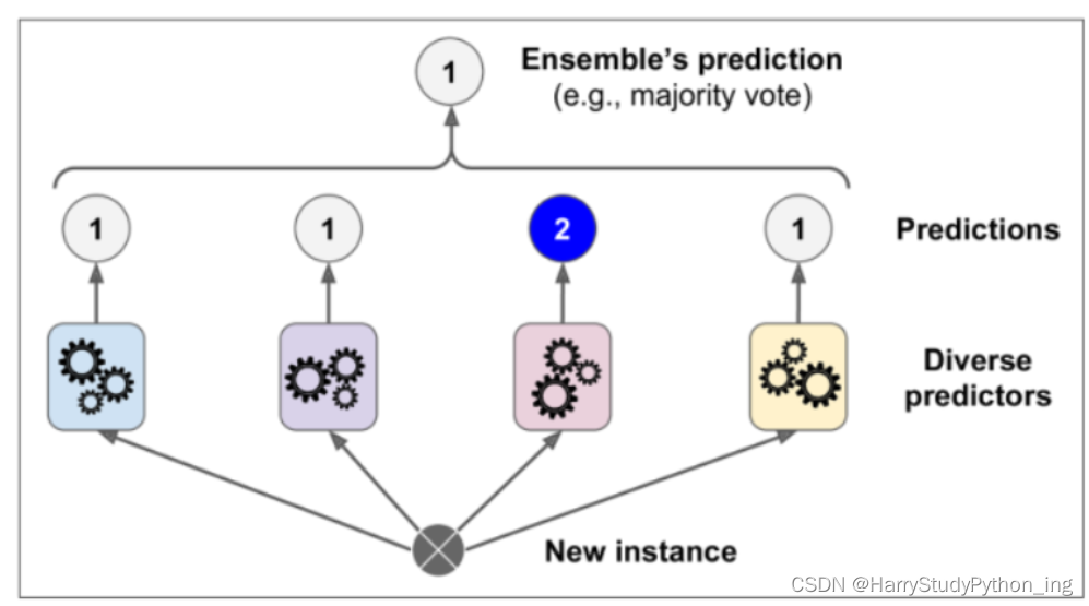
集成基本思想：

训练时用多种分类器一起完成同一份任务

测试时对待测试样本分别通过不同的分类器，汇总最后的结果

from sklearn.model_selection import train_test_split
from sklearn.datasets import make_moons

X,y = make_moons(n_samples=500, noise=0.30, random_state=42)
X_train, X_test, y_train, y_test = train_test_split(X, y, random_state=42)
plt.plot(X[:,0][y==0],X[:,1][y==0],'yo',alpha = 0.6)
plt.plot(X[:,0][y==0],X[:,1][y==1],'bs',alpha = 0.6)
1
2
3
4
5
6
7

投票策略：软投票与硬投票

• 硬投票：直接用类别值，少数服从多数
• 软投票：各自分类器的概率值进行加权平均

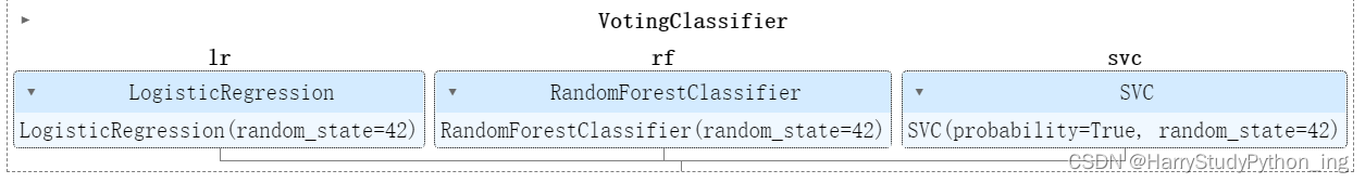
硬投票实验

from sklearn.ensemble import RandomForestClassifier, VotingClassifier
from sklearn.linear_model import LogisticRegression
from sklearn.svm import SVC

log_clf = LogisticRegression(random_state=42)
rnd_clf = RandomForestClassifier(random_state=42)
svm_clf = SVC(random_state=42)

voting_clf = VotingClassifier(estimators =[('lr',log_clf),('rf',rnd_clf),('svc',svm_clf)],voting='hard')
voting_clf.fit(X_train,y_train)
1
2
3
4
5
6
7
8
9
10

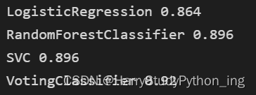
from sklearn.metrics import accuracy_score
for clf in (log_clf,rnd_clf,svm_clf,voting_clf):
    clf.fit(X_train,y_train)
    y_pred = clf.predict(X_test)
    print (clf.__class__.__name__,accuracy_score(y_test,y_pred))
1
2
3
4
5

软投票实验

from sklearn.ensemble import RandomForestClassifier, VotingClassifier
from sklearn.linear_model import LogisticRegression
from sklearn.svm import SVC

log_clf = LogisticRegression(random_state=42)
rnd_clf = RandomForestClassifier(random_state=42)
svm_clf = SVC(probability = True,random_state=42)

voting_clf = VotingClassifier(estimators =[('lr',log_clf),('rf',rnd_clf),('svc',svm_clf)],voting='soft')
voting_clf.fit(X_train,y_train)
1
2
3
4
5
6
7
8
9
10

from sklearn.metrics import accuracy_score
for clf in (log_clf,rnd_clf,svm_clf,voting_clf):
    clf.fit(X_train,y_train)
    y_pred = clf.predict(X_test)
    print (clf.__class__.__name__,accuracy_score(y_test,y_pred))
1
2
3
4
5

软投票：要求必须各个分别器都能得出概率值

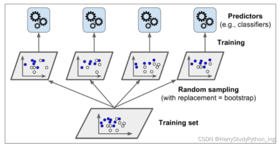
Bagging策略

• 首先对训练数据集进行多次采样，保证每次得到的采样数据都是不同的
• 分别训练多个模型，例如树模型
• 预测时需得到所有模型结果再进行集成
  

from sklearn.ensemble import BaggingClassifier
from sklearn.tree import DecisionTreeClassifier

bag_clf = BaggingClassifier(DecisionTreeClassifier(),
                  n_estimators = 500,
                  max_samples = 100,
                  bootstrap = True,
                  n_jobs = -1,
                  random_state = 42
)
bag_clf.fit(X_train,y_train)
y_pred = bag_clf.predict(X_test)
import sys
import codecs
sys.stdout = codecs.getwriter("utf-8")(sys.stdout)
1
2
3
4
5
6
7
8
9
10
11
12
13
14
15

accuracy_score(y_test,y_pred)
1

tree_clf = DecisionTreeClassifier(random_state = 42)
tree_clf.fit(X_train,y_train)
y_pred_tree = tree_clf.predict(X_test)
accuracy_score(y_test,y_pred_tree)
1
2
3
4

决策边界

• 集成与传统方法对比

from matplotlib.colors import ListedColormap
def plot_decision_boundary(clf,X,y,axes=[-1.5,2.5,-1,1.5],alpha=0.5,contour =True):
    x1s=np.linspace(axes[0],axes[1],100)
    x2s=np.linspace(axes[2],axes[3],100)
    x1,x2 = np.meshgrid(x1s,x2s)
    X_new = np.c_[x1.ravel(),x2.ravel()]
    y_pred = clf.predict(X_new).reshape(x1.shape)
    custom_cmap = ListedColormap(['#fafab0','#9898ff','#a0faa0'])
    plt.contourf(x1,x2,y_pred,cmap = custom_cmap,alpha=0.3)
    if contour:
        custom_cmap2 = ListedColormap(['#7d7d58','#4c4c7f','#507d50'])
        plt.contour(x1,x2,y_pred,cmap = custom_cmap2,alpha=0.8)
    plt.plot(X[:,0][y==0],X[:,1][y==0],'yo',alpha = 0.6)
    plt.plot(X[:,0][y==0],X[:,1][y==1],'bs',alpha = 0.6)
    plt.axis(axes)
    plt.xlabel('x1')
    plt.xlabel('x2')

plt.figure(figsize = (12,5))
plt.subplot(121)
plot_decision_boundary(tree_clf,X,y)
plt.title('Decision Tree')
plt.subplot(122)
plot_decision_boundary(bag_clf,X,y)
plt.title('Decision Tree With Bagging')
1
2
3
4
5
6
7
8
9
10
11
12
13
14
15
16
17
18
19
20
21
22
23
24
25

Colormap颜色：https://blog.csdn.net/zhaogeng111/article/details/78419015

OOB策略

• Out Of Bag

bag_clf = BaggingClassifier(DecisionTreeClassifier(),
                  n_estimators = 500,
                  max_samples = 100,
                  bootstrap = True,
                  n_jobs = -1,
                  random_state = 42,
                  oob_score = True
)
bag_clf.fit(X_train,y_train)
bag_clf.oob_score_
1
2
3
4
5
6
7
8
9
10

y_pred = bag_clf.predict(X_test)
accuracy_score(y_test,y_pred)
bag_clf.oob_decision_function_
1
2
3

随机森林

from sklearn.ensemble import RandomForestClassifier
rf_clf = RandomForestClassifier()
rf_clf.fit(X_train,y_train)
1
2
3

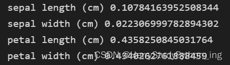
特征重要性：

sklearn中是看每个特征的平均深度

from sklearn.datasets import load_iris
iris = load_iris()
rf_clf = RandomForestClassifier(n_estimators=500,n_jobs=-1)
rf_clf.fit(iris['data'],iris['target'])
for name,score in zip(iris['feature_names'],rf_clf.feature_importances_):
    print (name,score)
1
2
3
4
5
6

Mnist中哪些特征比较重要呢？

from sklearn.datasets import fetch_openml
mnist = fetch_openml('mnist_784')
rf_clf = RandomForestClassifier(n_estimators=500,n_jobs=-1)
rf_clf.fit(mnist['data'],mnist['target'])

rf_clf.feature_importances_.shape
def plot_digit(data):
    image = data.reshape(28,28)
    plt.imshow(image,cmap=matplotlib.cm.hot)
    plt.axis('off')

plot_digit(rf_clf.feature_importances_)
char = plt.colorbar(ticks=[rf_clf.feature_importances_.min(),rf_clf.feature_importances_.max()])
char.ax.set_yticklabels(['Not important','Very important'])
1
2
3
4
5
6
7
8
9
10
11
12
13
14

Boosting-提升策略

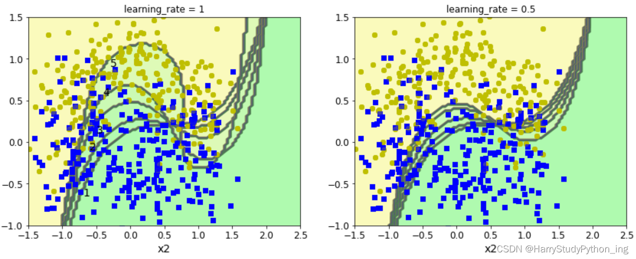
AdaBoost

跟上学时的考试一样，这次做错的题，是不是得额外注意，下次的时候就和别错了！

以SVM分类器为例来演示AdaBoost的基本策略

from sklearn.svm import SVC

m = len(X_train)

plt.figure(figsize=(14,5))
for subplot,learning_rate in ((121,1),(122,0.5)):
    sample_weights = np.ones(m)
    plt.subplot(subplot)
    for i in range(5):
        svm_clf = SVC(kernel='rbf',C=0.05,random_state=42)
        svm_clf.fit(X_train,y_train,sample_weight = sample_weights)
        y_pred = svm_clf.predict(X_train)
        sample_weights[y_pred != y_train] *= (1+learning_rate)
        plot_decision_boundary(svm_clf,X,y,alpha=0.2)
        plt.title('learning_rate = {}'.format(learning_rate))
    if subplot == 121:
        plt.text(-0.7, -0.65, "1", fontsize=14)
        plt.text(-0.6, -0.10, "2", fontsize=14)
        plt.text(-0.5,  0.10, "3", fontsize=14)
        plt.text(-0.4,  0.55, "4", fontsize=14)
        plt.text(-0.3,  0.90, "5", fontsize=14)
plt.show()
1
2
3
4
5
6
7
8
9
10
11
12
13
14
15
16
17
18
19
20
21
22

from sklearn.ensemble import AdaBoostClassifier
ada_clf = AdaBoostClassifier(DecisionTreeClassifier(max_depth=1),
                   n_estimators = 200,
                   learning_rate = 0.5,
                   random_state = 42
)
ada_clf.fit(X_train,y_train)
plot_decision_boundary(ada_clf,X,y)
1
2
3
4
5
6
7
8

Gradient Boosting

np.random.seed(42)
X = np.random.rand(100,1) - 0.5
y = 3*X[:,0]**2 + 0.05*np.random.randn(100)
y.shape
from sklearn.tree import DecisionTreeRegressor
tree_reg1 = DecisionTreeRegressor(max_depth = 2)
tree_reg1.fit(X,y)
y2 = y - tree_reg1.predict(X)
tree_reg2 = DecisionTreeRegressor(max_depth = 2)
tree_reg2.fit(X,y2)
y3 = y2 - tree_reg2.predict(X)
tree_reg3 = DecisionTreeRegressor(max_depth = 2)
tree_reg3.fit(X,y3)
X_new = np.array([[0.8]])
y_pred = sum(tree.predict(X_new) for tree in (tree_reg1,tree_reg2,tree_reg3))
y_pred
def plot_predictions(regressors, X, y, axes, label=None, style="r-", data_style="b.", data_label=None):
    x1 = np.linspace(axes[0], axes[1], 500)
    y_pred = sum(regressor.predict(x1.reshape(-1, 1)) for regressor in regressors)
    plt.plot(X[:, 0], y, data_style, label=data_label)
    plt.plot(x1, y_pred, style, linewidth=2, label=label)
    if label or data_label:
        plt.legend(loc="upper center", fontsize=16)
    plt.axis(axes)

plt.figure(figsize=(11,11))

plt.subplot(321)
plot_predictions([tree_reg1], X, y, axes=[-0.5, 0.5, -0.1, 0.8], label="$h_1(x_1)$", style="g-", data_label="Training set")
plt.ylabel("$y$", fontsize=16, rotation=0)
plt.title("Residuals and tree predictions", fontsize=16)

plt.subplot(322)
plot_predictions([tree_reg1], X, y, axes=[-0.5, 0.5, -0.1, 0.8], label="$h(x_1) = h_1(x_1)$", data_label="Training set")
plt.ylabel("$y$", fontsize=16, rotation=0)
plt.title("Ensemble predictions", fontsize=16)

plt.subplot(323)
plot_predictions([tree_reg2], X, y2, axes=[-0.5, 0.5, -0.5, 0.5], label="$h_2(x_1)$", style="g-", data_style="k+", data_label="Residuals")
plt.ylabel("$y - h_1(x_1)$", fontsize=16)

plt.subplot(324)
plot_predictions([tree_reg1, tree_reg2], X, y, axes=[-0.5, 0.5, -0.1, 0.8], label="$h(x_1) = h_1(x_1) + h_2(x_1)$")
plt.ylabel("$y$", fontsize=16, rotation=0)

plt.subplot(325)
plot_predictions([tree_reg3], X, y3, axes=[-0.5, 0.5, -0.5, 0.5], label="$h_3(x_1)$", style="g-", data_style="k+")
plt.ylabel("$y - h_1(x_1) - h_2(x_1)$", fontsize=16)
plt.xlabel("$x_1$", fontsize=16)

plt.subplot(326)
plot_predictions([tree_reg1, tree_reg2, tree_reg3], X, y, axes=[-0.5, 0.5, -0.1, 0.8], label="$h(x_1) = h_1(x_1) + h_2(x_1) + h_3(x_1)$")
plt.xlabel("$x_1$", fontsize=16)
plt.ylabel("$y$", fontsize=16, rotation=0)

plt.show()
1
2
3
4
5
6
7
8
9
10
11
12
13
14
15
16
17
18
19
20
21
22
23
24
25
26
27
28
29
30
31
32
33
34
35
36
37
38
39
40
41
42
43
44
45
46
47
48
49
50
51
52
53
54
55
56

from sklearn.ensemble import GradientBoostingRegressor
gbrt = GradientBoostingRegressor(max_depth = 2,
                          n_estimators = 3,
                          learning_rate = 1.0,
                          random_state = 41
)
gbrt.fit(X,y)
gbrt_slow_1 = GradientBoostingRegressor(max_depth = 2,
                          n_estimators = 3,
                          learning_rate = 0.1,
                          random_state = 41
)
gbrt_slow_1.fit(X,y)
gbrt_slow_2 = GradientBoostingRegressor(max_depth = 2,
                          n_estimators = 200,
                          learning_rate = 0.1,
                          random_state = 41
)
gbrt_slow_2.fit(X,y)
plt.figure(figsize = (11,4))
plt.subplot(121)
plot_predictions([gbrt],X,y,axes=[-0.5,0.5,-0.1,0.8],label = 'Ensemble predictions')
plt.title('learning_rate={},n_estimators={}'.format(gbrt.learning_rate,gbrt.n_estimators))

plt.subplot(122)
plot_predictions([gbrt_slow_1],X,y,axes=[-0.5,0.5,-0.1,0.8],label = 'Ensemble predictions')
plt.title('learning_rate={},n_estimators={}'.format(gbrt_slow_1.learning_rate,gbrt_slow_1.n_estimators))
1
2
3
4
5
6
7
8
9
10
11
12
13
14
15
16
17
18
19
20
21
22
23
24
25
26
27

plt.figure(figsize = (11,4))
plt.subplot(121)
plot_predictions([gbrt_slow_2],X,y,axes=[-0.5,0.5,-0.1,0.8],label = 'Ensemble predictions')
plt.title('learning_rate={},n_estimators={}'.format(gbrt_slow_2.learning_rate,gbrt_slow_2.n_estimators))

plt.subplot(122)
plot_predictions([gbrt_slow_1],X,y,axes=[-0.5,0.5,-0.1,0.8],label = 'Ensemble predictions')
plt.title('learning_rate={},n_estimators={}'.format(gbrt_slow_1.learning_rate,gbrt_slow_1.n_estimators))
1
2
3
4
5
6
7
8

提前停止策略

from sklearn.metrics import mean_squared_error
X_train,X_val,y_train,y_val = train_test_split(X,y,random_state=49)
gbrt = GradientBoostingRegressor(max_depth = 2,
                          n_estimators = 120,
                          random_state = 42
)
gbrt.fit(X_train,y_train)

errors = [mean_squared_error(y_val,y_pred) for y_pred in gbrt.staged_predict(X_val)]
bst_n_estimators = np.argmin(errors)

gbrt_best = GradientBoostingRegressor(max_depth = 2,
                          n_estimators = bst_n_estimators,
                          random_state = 42
)
gbrt_best.fit(X_train,y_train)
min_error = np.min(errors)
min_error
plt.figure(figsize = (11,4))
plt.subplot(121)
plt.plot(errors,'b.-')
plt.plot([bst_n_estimators,bst_n_estimators],[0,min_error],'k--')
plt.plot([0,120],[min_error,min_error],'k--')
plt.axis([0,120,0,0.01])
plt.title('Val Error')

plt.subplot(122)
plot_predictions([gbrt_best],X,y,axes=[-0.5,0.5,-0.1,0.8])
plt.title('Best Model(%d trees)'%bst_n_estimators)
1
2
3
4
5
6
7
8
9
10
11
12
13
14
15
16
17
18
19
20
21
22
23
24
25
26
27
28
29

gbrt = GradientBoostingRegressor(max_depth = 2,
                             random_state = 42,
                                 warm_start =True
)
error_going_up = 0
min_val_error = float('inf')

for n_estimators in range(1,120):
    gbrt.n_estimators = n_estimators
    gbrt.fit(X_train,y_train)
    y_pred = gbrt.predict(X_val)
    val_error = mean_squared_error(y_val,y_pred)
    if val_error < min_val_error:
        min_val_error = val_error
        error_going_up = 0
    else:
        error_going_up +=1
        if error_going_up == 5:
            break
        
print (gbrt.n_estimators)
1
2
3
4
5
6
7
8
9
10
11
12
13
14
15
16
17
18
19
20
21

Stacking（堆叠集成）

from sklearn.model_selection import train_test_split
from sklearn.datasets import fetch_openml
mnist = fetch_openml('mnist_784')

X_train_val, X_test, y_train_val, y_test = train_test_split(
    mnist.data, mnist.target, test_size=10000, random_state=42)
X_train, X_val, y_train, y_val = train_test_split(
    X_train_val, y_train_val, test_size=10000, random_state=42)
from sklearn.ensemble import RandomForestClassifier, ExtraTreesClassifier
from sklearn.svm import LinearSVC
from sklearn.neural_network import MLPClassifier
random_forest_clf = RandomForestClassifier(random_state=42)
extra_trees_clf = ExtraTreesClassifier(random_state=42)
svm_clf = LinearSVC(random_state=42)
mlp_clf = MLPClassifier(random_state=42)

estimators = [random_forest_clf, extra_trees_clf, svm_clf, mlp_clf]
for estimator in estimators:
    print("Training the", estimator)
    estimator.fit(X_train, y_train)
X_val_predictions = np.empty((len(X_val), len(estimators)), dtype=np.float32)

for index, estimator in enumerate(estimators):
    X_val_predictions[:, index] = estimator.predict(X_val)
    
X_val_predictions
rnd_forest_blender = RandomForestClassifier(n_estimators=200, oob_score=True, random_state=42)
rnd_forest_blender.fit(X_val_predictions, y_val)
rnd_forest_blender.oob_score_
1
2
3
4
5
6
7
8
9
10
11
12
13
14
15
16
17
18
19
20
21
22
23
24
25
26
27
28
29