实验数据集：全国工作情况数据集下载
运行工具：jupyter notebook

一、数据预处理

import pandas as pd
import numpy as np
from pyecharts.charts import *
from pyecharts import options as opts
from pyecharts.commons.utils import JsCode
from pyecharts.globals import SymbolType
from pyecharts.components import Table
import textwrap
1
2
3
4
5
6
7
8

path = r'2022年数据分析岗招聘数据.csv'#修改文件存储目录
data = pd.read_csv(path)
data.head()
1
2
3

# 城市数据处理
data['城市'] = data['地点'].apply(lambda x:x.split('-')[0])
data.head()
1
2
3

# 薪资数据处理
# 去除非范围类数据
data2 = data[data['薪资范围'] != '面议']
data2 = data2[~data2.薪资范围.str.contains('/天')]
data2 = data2[~data2.薪资范围.str.contains('以下')]
data2['薪资下限'] = data2.薪资范围.apply(lambda x:x.split('-')[0])
data2['薪资上限'] = data2.薪资范围.apply(lambda x:x.split('-')[1])
# 定义函数将薪资转化为数字形式
def salary_handle(word):
    if word[-1] == '万':
        num = float(word.strip('万')) * 10000
    elif word[-1] == '千':
        num = float(word.strip('千')) * 1000
    return num
data2['薪资下限'] = data2.薪资下限.apply(lambda x:salary_handle(x))
data2['薪资上限'] = data2.薪资上限.apply(lambda x:salary_handle(x))
data2['薪资均值'] = round((data2.薪资上限 + data2.薪资下限)/2,2)
data2.head()
1
2
3
4
5
6
7
8
9
10
11
12
13
14
15
16
17
18

print('不规范数据量为：',data.shape[0] - data2.shape[0])
1

不规范数据量为： 330

# 去除异常值
data2 = data2.reset_index(drop = True)
# data2[data2['工作经验']=='10年以上']
data2 = data2.drop(index = 5860)
1
2
3
4

在数据预处理部分，做了如下事情。

首先导入数据，查看数据基本情况。由于数据是自己爬的，所以每个字段的数据情况基本上都了解了，这部分就进行了省略。
然后处理城市数据。企业发布的招聘信息中，工作地点的信息大部分都精确到了具体的市区。因此这里将工作地区中的城市提取出来，方便后续统计。
然后对数据中的薪资范围进行处理。由于薪资范围的数据是‘1万-2万’或者是‘7千-9千’或者是'面议'或者是‘200元/天’这样的形式，因此要对薪资数据进行处理。查看薪资数据，发现大部分薪资的数据都是以‘7千-9千’这样的范围形式出现的，仅有少部分数据是‘面议’或者是‘200/天’这样的形式，这样不规范的数据总计330条，占比不是很大，因此将这部分数据直接进行去除。并且将范围中的7千、1万这样形式的数据都转换成具体的数值型数据，方便后续统计分析。并且去薪资的上限和下限的均值作为新字段进行分析。
1
2
3

二、岗位需求

1. 哪个城市的数据分析岗岗位需求较多呢？

我们首先来看看，哪个城市的数据分析岗的岗位需求最多呢？
绘制各城市岗位需求榜单如下。

# 绘制圆角柱状图函数
def echarts_bar(x,y,title = '主标题',subtitle = '副标题',label = '图例'):
    """
    x: 函数传入x轴标签数据
    y：函数传入y轴数据
    title：主标题
    subtitle：副标题
    label：图例
    """
    bar = Bar(
            init_opts=opts.InitOpts(
            # bg_color='#080b30',  # 设置背景颜色
            theme='shine',         # 设置主题
            width='1000px',     # 设置图的宽度
            height='700px'     # 设置图的高度
        )
    )
    bar.add_xaxis(x)
    bar.add_yaxis(label,y,
        label_opts=opts.LabelOpts(is_show=True) # 是否显示数据
        ,category_gap="50%" # 柱子宽度设置
        ) 
    bar.reversal_axis()
    bar.set_series_opts( # 自定义图表样式
        label_opts=opts.LabelOpts(
            is_show=True,
            position='right', # position 标签的位置 可选 'top'，'left'，'right'，'bottom'，'inside'，'insideLeft'，'insideRight'
            font_size=15,
            color= '#333333',
            font_weight = 'bolder',  # font_weight 文字字体的粗细  'normal'，'bold'，'bolder'，'lighter'
            font_style = 'oblique',  # font_style 文字字体的风格，可选 'normal'，'italic'，'oblique'
            ), # 是否显示数据标签
        itemstyle_opts={  
            "normal": {
                "color": JsCode(
                    """new echarts.graphic.LinearGradient(0, 0, 0, 1, [{
                        offset: 0,color: '#FC7D5D'}
                        ,{offset: 1,color: '#C45739'}], false)
                    """
                ),       # 调整柱子颜色渐变
                'shadowBlur': 6,   # 光影大小
                "barBorderRadius": [100, 100, 100, 100],  # 调整柱子圆角弧度
                "shadowColor": "#999999", # 调整阴影颜色
                'shadowOffsetY': 2,
                'shadowOffsetX': 2,  # 偏移量
            }
        }
    )
    bar.set_global_opts(
        # 标题设置
        title_opts=opts.TitleOpts(
            title=title, # 主标题
            subtitle=subtitle, # 副标题
            pos_left='center',  # 标题展示位置
            title_textstyle_opts=opts.TextStyleOpts(color='#2C3B4C', font_size=20,font_weight='bolder')
        ),
        # 图例设置
        legend_opts=opts.LegendOpts(
            is_show=True, # 是否显示图例
            pos_left='right', # 图例显示位置
            pos_top='3%',  #图例距离顶部的距离
            orient='horizontal'  # 图例水平布局
        ),
        tooltip_opts=opts.TooltipOpts(
            is_show=True,  # 是否使用提示框
            trigger='axis',  # 触发类型
            trigger_on='mousemove|click',  # 触发条件，点击或者悬停均可出发
            axis_pointer_type='cross',  # 指示器类型，鼠标移动到图表区可以查看效果
        ),
        yaxis_opts=opts.AxisOpts(
            is_show=True,
            splitline_opts=opts.SplitLineOpts(is_show=False), # 分割线
            axistick_opts=opts.AxisTickOpts(is_show=False), # 刻度不显示
            axislabel_opts=opts.LabelOpts(  # 坐标轴标签配置
                font_size=13,  # 字体大小
                font_weight='bolder' # 字重
            ),
        ),   # 关闭Y轴显示
        xaxis_opts=opts.AxisOpts(
            boundary_gap=True,    # 两边不显示间隔
            axistick_opts=opts.AxisTickOpts(is_show=True),  # 刻度不显示
            splitline_opts=opts.SplitLineOpts(is_show=False),  # 分割线不显示
            axisline_opts=opts.AxisLineOpts(is_show=True),  # 轴不显示
            axislabel_opts=opts.LabelOpts(  # 坐标轴标签配置
                font_size=13,  # 字体大小
                font_weight='bolder' # 字重
            ),
        ),
    )
    return bar
1
2
3
4
5
6
7
8
9
10
11
12
13
14
15
16
17
18
19
20
21
22
23
24
25
26
27
28
29
30
31
32
33
34
35
36
37
38
39
40
41
42
43
44
45
46
47
48
49
50
51
52
53
54
55
56
57
58
59
60
61
62
63
64
65
66
67
68
69
70
71
72
73
74
75
76
77
78
79
80
81
82
83
84
85
86
87
88
89
90

job_demand = data2.城市.value_counts().sort_values(ascending = True)
echarts_bar(job_demand.index.tolist(),job_demand.values.tolist(),title = '全国各地数据分析岗岗位需求排名',subtitle = ' ',
            label = '岗位需求量').render_notebook()
1
2
3

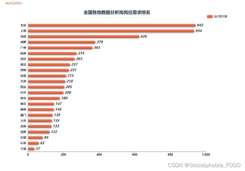通过全国各地数据分析岗岗位需求排名可以发现，北京上海的岗位需求是最多的。其次是深圳。在北上广深四个一线城市中，广州的数据分析岗位需求是最少的。而成都的数据分析岗的岗位需求量近几年增长较快，甚至超过了广州。其次是杭州、武汉、南京等城市。
因此要找数据分析岗工作或者实习的小伙伴，还是推荐去北上广深这样的一线城市。

2. 岗位需求较多的城市中，哪个区的岗位需求更多呢？

我们进一步查看北上广深以及成都、杭州等数据分析岗岗位需求排名前9的城市，其数据分析岗岗位需求主要分别分布在哪些区。

# 北上广深和成都杭州各个地区岗位需求量
beijing_demand = data[data['城市'] == '北京']['地点'].value_counts().sort_values(ascending = False)
shanghai_demand = data[data['城市'] == '上海']['地点'].value_counts().sort_values(ascending = False)
shenzhen_demand = data[data['城市'] == '深圳']['地点'].value_counts().sort_values(ascending = False)
guangzhou_demand = data[data['城市'] == '广州']['地点'].value_counts().sort_values(ascending = False)
chengdu_demand = data[data['城市'] == '成都']['地点'].value_counts().sort_values(ascending = False)
hangzhou_demand = data[data['城市'] == '杭州']['地点'].value_counts().sort_values(ascending = False)
1
2
3
4
5
6
7

def bar_chart(desc, title_pos):
    df_t = data[(data['城市'] == desc)&(data['地点'] != desc)]['地点'].value_counts().sort_values(ascending = False).reset_index()
    df_t.columns = [desc,'岗位需求量']
    df_t[desc] = df_t[desc].apply(lambda x:x.split('-')[1])
    # 新建一个Bar
    chart = Bar(
        init_opts=opts.InitOpts(
            # bg_color='#2C3B4C',  # 设置背景颜色
            theme='white',         # 设置主题
            width='400px',     # 设置图的宽度
            height='400px'
        )
    )
    chart.add_xaxis(
        df_t[desc].tolist()
    )
    chart.add_yaxis(
        '',
        df_t['岗位需求量'].tolist()
    )
    chart.set_series_opts( # 自定义图表样式
        label_opts=opts.LabelOpts(
            is_show=True,
            position='top', # position 标签的位置 可选 'top'，'left'，'right'，'bottom'，'inside'，'insideLeft'，'insideRight'
            font_size=15,
            color= '#727F91',
            font_weight = 'bolder',  # font_weight 文字字体的粗细  'normal'，'bold'，'bolder'，'lighter'
            font_style = 'oblique',  # font_style 文字字体的风格，可选 'normal'，'italic'，'oblique'
            ), # 是否显示数据标签
        itemstyle_opts={  
            "normal": {
                'shadowBlur': 10,   # 光影大小
                "barBorderRadius": [100, 100, 0, 0],  # 调整柱子圆角弧度
                "shadowColor": "#94A4B4", # 调整阴影颜色
                'shadowOffsetY': 6,
                'shadowOffsetX': 6,  # 偏移量
            }
        }
    )
    # Bar的全局配置项
    chart.set_global_opts(
        xaxis_opts=opts.AxisOpts(
            name='地区',
            is_scale=True,
            axislabel_opts=opts.LabelOpts(rotate = 45),
            # 网格线配置
            splitline_opts=opts.SplitLineOpts(
                is_show=False,
                linestyle_opts=opts.LineStyleOpts(
                    type_='dashed'))
        ),
        yaxis_opts=opts.AxisOpts(
            is_scale=True,
            name='岗位需求量',
            type_="value",
            # 网格线配置
            splitline_opts=opts.SplitLineOpts(
                is_show=False,
                linestyle_opts=opts.LineStyleOpts(
                    type_='dashed'))
        ),
        # 标题配置
        title_opts=opts.TitleOpts(
            title=desc,
            pos_left=title_pos[0],
            pos_top=title_pos[1],
            title_textstyle_opts=opts.TextStyleOpts(color='#2C3B4C', font_size=20)
        ),
        tooltip_opts=opts.TooltipOpts(
            is_show=True,  # 是否使用提示框
            trigger='axis',  # 触发类型
            # is_show_content = True,
            trigger_on='mousemove|click',  # 触发条件，点击或者悬停均可出发
            axis_pointer_type='cross',  # 指示器类型，鼠标移动到图表区可以查看效果
        ),
    )
    return chart

grid = Grid(
    init_opts=opts.InitOpts(
        theme='white',
        width='1200px',
        height='1200px',
        )
)
# 依次添加不同属性下价格对比Bar
grid.add(
    bar_chart('北京', ['15%', '3%']),
    # is_control_axis_index=False,
    grid_opts=opts.GridOpts(
        pos_top='10%',   # 指定Grid中子图的位置
        pos_bottom='70%',
        pos_left='5%',
        pos_right='70%'
    )
)
grid.add(
    bar_chart('上海', ['50%', '3%']),
    # is_control_axis_index=False,
    grid_opts=opts.GridOpts(
        pos_top='10%',
        pos_bottom='70%',
        pos_left='40%',
        pos_right='35%'
    )
)
grid.add(
    bar_chart('广州', ['85%', '3%']),
    # is_control_axis_index=False,
    grid_opts=opts.GridOpts(
        pos_top='10%',
        pos_bottom='70%',
        pos_left='75%',
        pos_right='0%'
    )
)
grid.add(
    bar_chart('深圳', ['15%', '33%']),
    # is_control_axis_index=False,
    grid_opts=opts.GridOpts(
        pos_top='40%',
        pos_bottom='40%',
        pos_left='5%',
        pos_right='70%'
    )
)
grid.add(
    bar_chart('成都', ['50%', '33%']),
    # is_control_axis_index=False,
    grid_opts=opts.GridOpts(
        pos_top='40%',
        pos_bottom='40%',
        pos_left='40%',
        pos_right='35%'
    )
)
grid.add(
    bar_chart('杭州', ['85%', '33%']),
    # is_control_axis_index=False,
    grid_opts=opts.GridOpts(
        pos_top='40%',
        pos_bottom='40%',
        pos_left='75%',
        pos_right='0%'
    )
)
grid.add(
    bar_chart('武汉', ['15%', '63%']),
    # is_control_axis_index=False,
    grid_opts=opts.GridOpts(
        pos_top='70%',
        pos_bottom='10%',
        pos_left='5%',
        pos_right='70%'
    )
)
grid.add(
    bar_chart('南京', ['50%', '63%']),
    # is_control_axis_index=False,
    grid_opts=opts.GridOpts(
        pos_top='70%',
        pos_bottom='10%',
        pos_left='40%',
        pos_right='35%'
    )
)
grid.add(
    bar_chart('郑州', ['85%', '63%']),
    # is_control_axis_index=False,
    grid_opts=opts.GridOpts(
        pos_top='70%',
        pos_bottom='10%',
        pos_left='75%',
        pos_right='0%'
    )
)
grid.render_notebook()
1
2
3
4
5
6
7
8
9
10
11
12
13
14
15
16
17
18
19
20
21
22
23
24
25
26
27
28
29
30
31
32
33
34
35
36
37
38
39
40
41
42
43
44
45
46
47
48
49
50
51
52
53
54
55
56
57
58
59
60
61
62
63
64
65
66
67
68
69
70
71
72
73
74
75
76
77
78
79
80
81
82
83
84
85
86
87
88
89
90
91
92
93
94
95
96
97
98
99
100
101
102
103
104
105
106
107
108
109
110
111
112
113
114
115
116
117
118
119
120
121
122
123
124
125
126
127
128
129
130
131
132
133
134
135
136
137
138
139
140
141
142
143
144
145
146
147
148
149
150
151
152
153
154
155
156
157
158
159
160
161
162
163
164
165
166
167
168
169
170
171
172
173
174
175
176
177

通过绘制柱状图可以发现，北京作为岗位需求最多的城市，其数据分析岗主要分布在朝阳区和海淀区，而其他区仅有这两个区的不到三分之一的岗位需求。
上海数据分析岗岗位需求最多的区是浦东新区，其次是徐汇区，而徐汇区的岗位需求也不及浦东新区的一半。
广州的数据分析岗岗位需求主要分布在天河区，海珠越秀黄埔也有一部分数据分析岗，但是最主要的还是再天河区。
深圳的数据分析岗岗位需求主要分布在南山区、福田区以及龙岗区。
…

三、薪资

下边看大部分小伙伴都比较关心的问题，就是薪资水平。这里的计算采用的都是企业发布的招聘的薪资范围的均值。

1. 各个城市平均薪资水平排名

city_salary = data2[['城市','薪资均值']].groupby('城市').mean().round(0).sort_values(by = '薪资均值',ascending = True).reset_index()
echarts_bar(city_salary['城市'].tolist(),city_salary['薪资均值'].tolist(),title = '全国各城市数据分析岗平均薪资水平排名',
            subtitle = '',label = '平均薪资').render_notebook()
1
2
3

查看各个城市的薪资水平可以发现，北上广深身为经济最发达的四个一线城市，薪资水平也是最高的。数据分析岗薪资最高的城市是上海，而四个城市中薪资最低的城市是广州。南京和苏杭二州的薪资是紧随其后的，值得一提的是，岗位需求量超过广州的成都，薪资水平却处于中等水平。

2. 各工作经验和学历的薪资水平对比

知道了哪个城市薪资水平较高以后，我们看看不同工作经验和不同学历的薪资水平分布是怎么样的吧

# 不同学历、不同经验、大专-不同经验交叉分析、本科-不同经验交叉分析、硕士-不同经验交叉分析、学历不限-不同经验交叉分析
job_exp = data2[['工作经验','薪资均值']].groupby('工作经验').mean().round(0).sort_values(by = '薪资均值',ascending = False).reset_index()
job_edu = data2[['学历要求','薪资均值']].groupby('学历要求').mean().round(0).sort_values(by = '薪资均值',ascending = False).reset_index()
benke_exp = data2[data2['学历要求'] == '本科'][['工作经验','薪资均值']].groupby('工作经验').mean().round(0).\
            sort_values(by = '薪资均值',ascending = False).reset_index()
dazhuan_exp = data2[data2['学历要求'] == '大专'][['工作经验','薪资均值']].groupby('工作经验').mean().round(0).\
            sort_values(by = '薪资均值',ascending = False).reset_index()
shuoshi_exp = data2[data2['学历要求'] == '硕士'][['工作经验','薪资均值']].groupby('工作经验').mean().round(0).\
            sort_values(by = '薪资均值',ascending = False).reset_index()
buxian_exp = data2[data2['学历要求'] == '学历不限'][['工作经验','薪资均值']].groupby('工作经验').mean().round(0).\
            sort_values(by = '薪资均值',ascending = False).reset_index()
boshi_exp = data2[data2['学历要求'] == '博士'][['工作经验','薪资均值']].groupby('工作经验').mean().round(0).\
            sort_values(by = '薪资均值',ascending = False).reset_index()
gaozhong_exp = data2[data2['学历要求'] == '高中'][['工作经验','薪资均值']].groupby('工作经验').mean().round(0).\
            sort_values(by = '薪资均值',ascending = False).reset_index()
zhongzhuan_exp = data2[data2['学历要求'] == '中专/中技'][['工作经验','薪资均值']].groupby('工作经验').mean().round(0).\
            sort_values(by = '薪资均值',ascending = False).reset_index()
1
2
3
4
5
6
7
8
9
10
11
12
13
14
15
16
17

def bar_chart2(x,y,title_pos,title = '主标题',subtitle = '副标题'):
    # 新建一个Bar
    chart = Bar(
        init_opts=opts.InitOpts(
            # bg_color='#2C3B4C',  # 设置背景颜色
            theme='white',         # 设置主题
            width='400px',     # 设置图的宽度
            height='400px'
        )
    )
    chart.add_xaxis(
        x
    )
    chart.add_yaxis(
        '',
        y
    )
    chart.set_series_opts( # 自定义图表样式
        label_opts=opts.LabelOpts(
            is_show=True,
            position='top', # position 标签的位置 可选 'top'，'left'，'right'，'bottom'，'inside'，'insideLeft'，'insideRight'
            font_size=15,
            color= '#727F91',
            font_weight = 'bolder',  # font_weight 文字字体的粗细  'normal'，'bold'，'bolder'，'lighter'
            font_style = 'oblique',  # font_style 文字字体的风格，可选 'normal'，'italic'，'oblique'
            ), # 是否显示数据标签
        itemstyle_opts={  
            "normal": {
                'shadowBlur': 10,   # 光影大小
                "barBorderRadius": [100, 100, 0, 0],  # 调整柱子圆角弧度
                "shadowColor": "#94A4B4", # 调整阴影颜色
                'shadowOffsetY': 6,
                'shadowOffsetX': 6,  # 偏移量
            }
        }
    )
    # Bar的全局配置项
    chart.set_global_opts(
        xaxis_opts=opts.AxisOpts(
            name=' ',
            is_scale=True,
            axislabel_opts=opts.LabelOpts(rotate = 45),
            # 网格线配置
            splitline_opts=opts.SplitLineOpts(
                is_show=False,
                linestyle_opts=opts.LineStyleOpts(
                    type_='dashed'))
        ),
        yaxis_opts=opts.AxisOpts(
            is_scale=True,
            name='薪资均值',
            type_="value",
            # 网格线配置
            splitline_opts=opts.SplitLineOpts(
                is_show=False,
                linestyle_opts=opts.LineStyleOpts(
                    type_='dashed'))
        ),
        # 标题配置
        title_opts=opts.TitleOpts(
            title=title,
            subtitle = subtitle,
            pos_left=title_pos[0],
            pos_top=title_pos[1],
            title_textstyle_opts=opts.TextStyleOpts(color='#2C3B4C', font_size=20)
        ),
        tooltip_opts=opts.TooltipOpts(
            is_show=True,  # 是否使用提示框
            trigger='axis',  # 触发类型
            # is_show_content = True,
            trigger_on='mousemove|click',  # 触发条件，点击或者悬停均可出发
            axis_pointer_type='cross',  # 指示器类型，鼠标移动到图表区可以查看效果
        ),
    )
    return chart
1
2
3
4
5
6
7
8
9
10
11
12
13
14
15
16
17
18
19
20
21
22
23
24
25
26
27
28
29
30
31
32
33
34
35
36
37
38
39
40
41
42
43
44
45
46
47
48
49
50
51
52
53
54
55
56
57
58
59
60
61
62
63
64
65
66
67
68
69
70
71
72
73
74
75

grid = Grid(
    init_opts=opts.InitOpts(
        theme='white',
        width='1200px',
        height='1200px',
    )
)
# 依次添加不同属性下价格对比Bar
grid.add(
    bar_chart2(job_exp['工作经验'].tolist(), job_exp['薪资均值'].tolist(), ['15%', '3%'], title='不同工作经验薪资对比',
               subtitle=' '),
    grid_opts=opts.GridOpts(
        pos_top='10%',   # 指定Grid中子图的位置
        pos_bottom='70%',
        pos_left='5%',
        pos_right='70%'
    )
)
grid.add(
    bar_chart2(job_edu['学历要求'].tolist(), job_edu['薪资均值'].tolist(), ['50%', '3%'], title='不同学历要求薪资对比',
               subtitle=' '),
    grid_opts=opts.GridOpts(
        pos_top='10%',
        pos_bottom='70%',
        pos_left='40%',
        pos_right='35%'
    )
)
grid.add(
    bar_chart2(buxian_exp['工作经验'].tolist(), buxian_exp['薪资均值'].tolist(), ['85%', '3%'], title='学历不限',
               subtitle=' '),
    grid_opts=opts.GridOpts(
        pos_top='10%',
        pos_bottom='70%',
        pos_left='75%',
        pos_right='0%'
    )
)
grid.add(
    bar_chart2(dazhuan_exp['工作经验'].tolist(), dazhuan_exp['薪资均值'].tolist(), ['15%', '33%'], title='大专',
               subtitle=' '),
    grid_opts=opts.GridOpts(
        pos_top='40%',
        pos_bottom='40%',
        pos_left='5%',
        pos_right='70%'
    )
)
grid.add(
    bar_chart2(benke_exp['工作经验'].tolist(), benke_exp['薪资均值'].tolist(), ['50%', '33%'], title='本科',
               subtitle=' '),
    grid_opts=opts.GridOpts(
        pos_top='40%',
        pos_bottom='40%',
        pos_left='40%',
        pos_right='35%'
    )
)
grid.add(
    bar_chart2(shuoshi_exp['工作经验'].tolist(), shuoshi_exp['薪资均值'].tolist(), ['85%', '33%'], title='硕士',
               subtitle=' '),
    grid_opts=opts.GridOpts(
        pos_top='40%',
        pos_bottom='40%',
        pos_left='75%',
        pos_right='0%'
    )
)
grid.add(
    bar_chart2(boshi_exp['工作经验'].tolist(), boshi_exp['薪资均值'].tolist(), ['15%', '63%'], title='博士',
               subtitle=' '),
    grid_opts=opts.GridOpts(
        pos_top='70%',
        pos_bottom='10%',
        pos_left='5%',
        pos_right='70%'
    )
)
grid.add(
    bar_chart2(gaozhong_exp['工作经验'].tolist(), gaozhong_exp['薪资均值'].tolist(), ['50%', '63%'], title='高中',
               subtitle=' '),
    grid_opts=opts.GridOpts(
        pos_top='70%',
        pos_bottom='10%',
        pos_left='40%',
        pos_right='35%'
    )
)
grid.add(
    bar_chart2(zhongzhuan_exp['工作经验'].tolist(), zhongzhuan_exp['薪资均值'].tolist(), ['85%', '63%'], title='中专/中技',
               subtitle=' '),
    grid_opts=opts.GridOpts(
        pos_top='70%',
        pos_bottom='10%',
        pos_left='75%',
        pos_right='0%'
    )
)
grid.render_notebook()

1
2
3
4
5
6
7
8
9
10
11
12
13
14
15
16
17
18
19
20
21
22
23
24
25
26
27
28
29
30
31
32
33
34
35
36
37
38
39
40
41
42
43
44
45
46
47
48
49
50
51
52
53
54
55
56
57
58
59
60
61
62
63
64
65
66
67
68
69
70
71
72
73
74
75
76
77
78
79
80
81
82
83
84
85
86
87
88
89
90
91
92
93
94
95
96
97
98
99
100

总的来看工作经验、学历和薪资的关系，可以发现，工作经验和学历越高，相应的薪资也越高，这是毋庸置疑的。
通过不同学历背景下，不同的工作经验与薪资的交叉分析，不难看出，学历越高，相应的薪资的上升空间也是越高的。

3. 各城市不同工作经验薪资水平对比

def bar_chart(desc, title_pos):
    df_t = data2[data2['城市'] == desc][['工作经验','薪资均值']].groupby('工作经验').mean().round(0).sort_values(by = '薪资均值',
            ascending = False).reset_index()
    # 新建一个Bar
    chart = Bar(
        init_opts=opts.InitOpts(
            # bg_color='#2C3B4C',  # 设置背景颜色
            theme='white',         # 设置主题
            width='400px',     # 设置图的宽度
            height='400px'
        )
    )
    chart.add_xaxis(
        df_t['工作经验'].tolist()
    )
    chart.add_yaxis(
        '',
        df_t['薪资均值'].tolist()
    )
    chart.set_series_opts( # 自定义图表样式
        label_opts=opts.LabelOpts(
            is_show=True,
            position='top', # position 标签的位置 可选 'top'，'left'，'right'，'bottom'，'inside'，'insideLeft'，'insideRight'
            font_size=15,
            color= '#727F91',
            font_weight = 'bolder',  # font_weight 文字字体的粗细  'normal'，'bold'，'bolder'，'lighter'
            font_style = 'oblique',  # font_style 文字字体的风格，可选 'normal'，'italic'，'oblique'
            ), # 是否显示数据标签
        itemstyle_opts={  
            "normal": {
                'shadowBlur': 10,   # 光影大小
                "barBorderRadius": [100, 100, 0, 0],  # 调整柱子圆角弧度
                "shadowColor": "#94A4B4", # 调整阴影颜色
                'shadowOffsetY': 6,
                'shadowOffsetX': 6,  # 偏移量
            }
        }
    )
    # Bar的全局配置项
    chart.set_global_opts(
        xaxis_opts=opts.AxisOpts(
            name='工作经验',
            is_scale=True,
            axislabel_opts=opts.LabelOpts(rotate = 45),
            # 网格线配置
            splitline_opts=opts.SplitLineOpts(
                is_show=False,
                linestyle_opts=opts.LineStyleOpts(
                    type_='dashed'))
        ),
        yaxis_opts=opts.AxisOpts(
            is_scale=True,
            name='薪资均值',
            type_="value",
            # 网格线配置
            splitline_opts=opts.SplitLineOpts(
                is_show=False,
                linestyle_opts=opts.LineStyleOpts(
                    type_='dashed'))
        ),
        # 标题配置
        title_opts=opts.TitleOpts(
            title=desc,
            pos_left=title_pos[0],
            pos_top=title_pos[1],
            title_textstyle_opts=opts.TextStyleOpts(color='#2C3B4C', font_size=20)
        ),
        tooltip_opts=opts.TooltipOpts(
            is_show=True,  # 是否使用提示框
            trigger='axis',  # 触发类型
            # is_show_content = True,
            trigger_on='mousemove|click',  # 触发条件，点击或者悬停均可出发
            axis_pointer_type='cross',  # 指示器类型，鼠标移动到图表区可以查看效果
        ),
    )
    return chart

grid = Grid(
    init_opts=opts.InitOpts(
        theme='white',
        width='1200px',
        height='1200px',
        )
)
# 依次添加不同属性下价格对比Bar
grid.add(
    bar_chart('北京', ['15%', '3%']),
    # is_control_axis_index=False,
    grid_opts=opts.GridOpts(
        pos_top='10%',   # 指定Grid中子图的位置
        pos_bottom='70%',
        pos_left='5%',
        pos_right='70%'
    )
)
grid.add(
    bar_chart('上海', ['50%', '3%']),
    # is_control_axis_index=False,
    grid_opts=opts.GridOpts(
        pos_top='10%',
        pos_bottom='70%',
        pos_left='40%',
        pos_right='35%'
    )
)
grid.add(
    bar_chart('广州', ['85%', '3%']),
    # is_control_axis_index=False,
    grid_opts=opts.GridOpts(
        pos_top='10%',
        pos_bottom='70%',
        pos_left='75%',
        pos_right='0%'
    )
)
grid.add(
    bar_chart('深圳', ['15%', '33%']),
    # is_control_axis_index=False,
    grid_opts=opts.GridOpts(
        pos_top='40%',
        pos_bottom='40%',
        pos_left='5%',
        pos_right='70%'
    )
)
grid.add(
    bar_chart('成都', ['50%', '33%']),
    # is_control_axis_index=False,
    grid_opts=opts.GridOpts(
        pos_top='40%',
        pos_bottom='40%',
        pos_left='40%',
        pos_right='35%'
    )
)
grid.add(
    bar_chart('杭州', ['85%', '33%']),
    # is_control_axis_index=False,
    grid_opts=opts.GridOpts(
        pos_top='40%',
        pos_bottom='40%',
        pos_left='75%',
        pos_right='0%'
    )
)
grid.add(
    bar_chart('武汉', ['15%', '63%']),
    # is_control_axis_index=False,
    grid_opts=opts.GridOpts(
        pos_top='70%',
        pos_bottom='10%',
        pos_left='5%',
        pos_right='70%'
    )
)
grid.add(
    bar_chart('南京', ['50%', '63%']),
    # is_control_axis_index=False,
    grid_opts=opts.GridOpts(
        pos_top='70%',
        pos_bottom='10%',
        pos_left='40%',
        pos_right='35%'
    )
)
grid.add(
    bar_chart('郑州', ['85%', '63%']),
    # is_control_axis_index=False,
    grid_opts=opts.GridOpts(
        pos_top='70%',
        pos_bottom='10%',
        pos_left='75%',
        pos_right='0%'
    )
)
grid.render_notebook()
1
2
3
4
5
6
7
8
9
10
11
12
13
14
15
16
17
18
19
20
21
22
23
24
25
26
27
28
29
30
31
32
33
34
35
36
37
38
39
40
41
42
43
44
45
46
47
48
49
50
51
52
53
54
55
56
57
58
59
60
61
62
63
64
65
66
67
68
69
70
71
72
73
74
75
76
77
78
79
80
81
82
83
84
85
86
87
88
89
90
91
92
93
94
95
96
97
98
99
100
101
102
103
104
105
106
107
108
109
110
111
112
113
114
115
116
117
118
119
120
121
122
123
124
125
126
127
128
129
130
131
132
133
134
135
136
137
138
139
140
141
142
143
144
145
146
147
148
149
150
151
152
153
154
155
156
157
158
159
160
161
162
163
164
165
166
167
168
169
170
171
172
173
174
175
176

看各城市相应的薪资下限和上限，可以发现，北上广深的下限和上限都是很高的，做数据分析去一线城市是没毛病的~

四、岗位要求

1. 数据分析岗对工作经验和学历的需求情况

了解了薪资以后，接下来我们看下数据分析岗有哪些岗位需求吧~

pie1 = data[['工作经验','职位名称']].groupby('工作经验').count().sort_values(by = '职位名称',ascending = False).reset_index()
pie2 = data[['学历要求','职位名称']].groupby('学历要求').count().sort_values(by = '职位名称',ascending = False).reset_index()
pie1 = (Pie()
       .add('', [list(z) for z in zip(pie1['工作经验'], pie1['职位名称'])])
       .set_global_opts(
            title_opts=opts.TitleOpts(
                title='工作经验需求量',
                title_textstyle_opts=opts.TextStyleOpts(color='#2C3B4C', font_size=20)
        )
       )
       )
pie2 = (Pie()
       .add('', [list(z) for z in zip(pie2['学历要求'], pie2['职位名称'])])
       .set_global_opts(
            title_opts=opts.TitleOpts(
                title='学历需求量',
                title_textstyle_opts=opts.TextStyleOpts(color='#2C3B4C', font_size=20)
        )
       )
       )
page = Page()
page.add(pie1,pie2)
page.render_notebook()
1
2
3
4
5
6
7
8
9
10
11
12
13
14
15
16
17
18
19
20
21
22
23

首先看工作经验。数据分析岗在工作经验的要求上边，1-3年工作经验是最多的，而不限工作经验和3-5年工作经验的需求也相对较多。
在学历需求上边，本科和大专占了绝大部分，仅有较少一部分是要求硕士和博士学历的。因此数据分析岗对于学历的要求并不是很高。

2. 数据分析岗技能需求

接下来我们看下数据分析岗要具备哪些技能吧~
这里的数据是爬取自公司发布的职位信息中的职位标签，而非岗位JD

tag_array = data['岗位标签'].apply(lambda x:eval(x)).tolist()
tag_lis = []
for tag in tag_array:
    tag_lis += tag
tag_df = pd.DataFrame(tag_lis,columns = ['职位标签'])
tag_df_cnt = tag_df['职位标签'].value_counts().reset_index()
tag_df_cnt.columns = ['职位标签','计数']
word_cnt_lis = [tag for tag in zip(tag_df_cnt['职位标签'],tag_df_cnt['计数'])]
wc = (
    WordCloud()
    .add("",
    word_cnt_lis,
    )
    .set_global_opts(
        title_opts=opts.TitleOpts(title="岗位标签词云图"),
    )
)

wc.render_notebook()
1
2
3
4
5
6
7
8
9
10
11
12
13
14
15
16
17
18
19

绘制词云图我们可以发现，众多的岗位标签中，出现次数最频繁的就是python和sql了，因此可以说明，sql和python是数据分析岗必备的技能，当然excel技能在日常工作中使用同样很频繁。
词云中数据挖掘、数据清洗、SPSS、BI工具等一些词汇出现的也较多，具体的还要看各岗位的具体需求。

五、公司情况

1. 公司类型、公司规模统计

接下来我们看看招聘数据分析岗的企业中，主要都是哪些类型的企业，以及公司规模都是如何的。

company_type_cnt = data[['公司类型','公司规模']].groupby('公司类型').count().sort_values(by = '公司规模',ascending = False).reset_index()
# 删除空值
company_type_cnt = company_type_cnt.drop(index = 10)
company_type_cnt.columns = ['公司类型','数量']
company_size_cnt = data[['公司类型','公司规模']].groupby('公司规模').count().sort_values(by = '公司类型',ascending = False).reset_index()
company_size_cnt.columns = ['公司规模','数量']
pie1 = (Pie()
       .add('', [list(z) for z in zip(company_type_cnt['公司类型'], company_type_cnt['数量'])])
       .set_global_opts(
            title_opts=opts.TitleOpts(
                title='各类型公司数据分析岗需求量',
                title_textstyle_opts=opts.TextStyleOpts(color='#2C3B4C', font_size=20)
        )
       )
       )
pie2 = (Pie()
       .add('', [list(z) for z in zip(company_size_cnt['公司规模'], company_size_cnt['数量'])])
       .set_global_opts(
            title_opts=opts.TitleOpts(
                title='各规模公司数据分析岗需求量',
                title_textstyle_opts=opts.TextStyleOpts(color='#2C3B4C', font_size=20)
        )
       )
       )
page = Page()
page.add(pie1,pie2)
page.render_notebook()
1
2
3
4
5
6
7
8
9
10
11
12
13
14
15
16
17
18
19
20
21
22
23
24
25
26
27

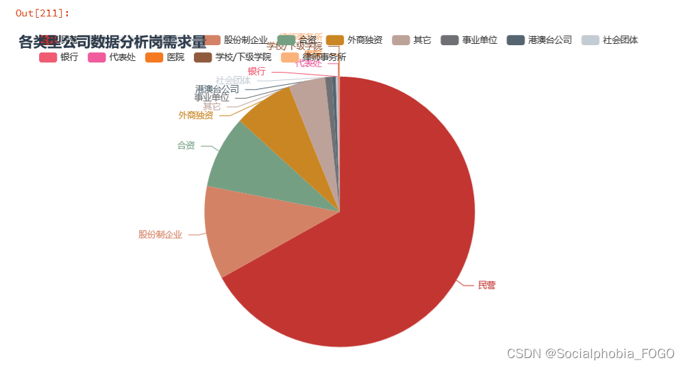
我们可以发现，招聘数据分析岗的企业中，以民营企业为主，占了一大半以上。
公司规模以1000-9999以及10000人以上的大型企业为主，大厂的数字化建设较为完善和成熟，因此会有较多的数据分析需求。同样也有部分中小企业，有可能是一些外包企业等。

2. 公司薪资待遇综合排名top50

接下来，我们统计出薪资待遇top前50的企业，希望可以为各位小伙伴提供一些参考的依据~

company_rank = data2[['职位名称','公司名称','薪资均值','公司规模']].groupby(['公司名称','公司规模','职位名称']).mean().\
                sort_values(by = ['薪资均值'],ascending = False).reset_index()
table = Table()
table_rows = [company_rank.iloc[i,:].tolist() for i in range(50)]
table.add(company_rank.columns.tolist(), table_rows)
table.render_notebook()
1
2
3
4
5
6