[R] ggplot2 - exercise (“fill =“)

We have made the plots like:

 Let's practice with what we have learnt in: [R] How to communicate with your data? - ggplot2-CSDN博客https://blog.csdn.net/m0_74331272/article/details/136513694

#tutorial 5 -script
#Exercise 1
#1.1#
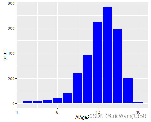
ggplot(smoking_and_drug_use_amongst_English_pupils,aes(x=AlAge2))+geom_histogram(fill="Blue",stat="count")
#1.2
ggplot(smoking_and_drug_use_amongst_English_pupils,aes(x=AlAge2))+geom_histogram(fill="Blue",stat="count", alpha=0.75)+labs(title="Age at which English pupils drunk alcohol for the first time",x="Age")
 
 
#Exercise 2
#2.1
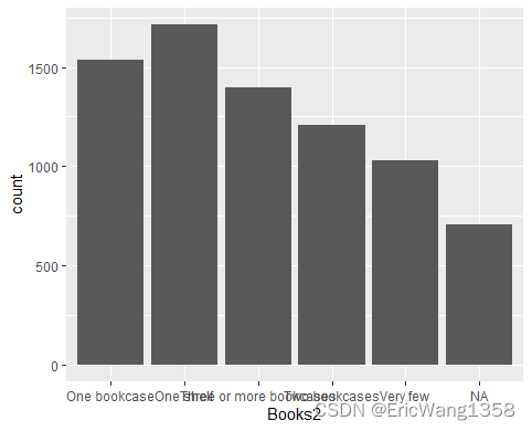
ggplot(smoking_and_drug_use_amongst_English_pupils,aes(x=Books2))+geom_bar()
#2.2 
ggplot(smoking_and_drug_use_amongst_English_pupils,aes(fct_infreq(Books2)))+geom_bar()
 
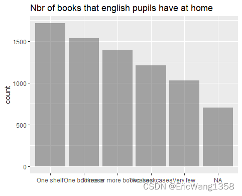
#.2.3
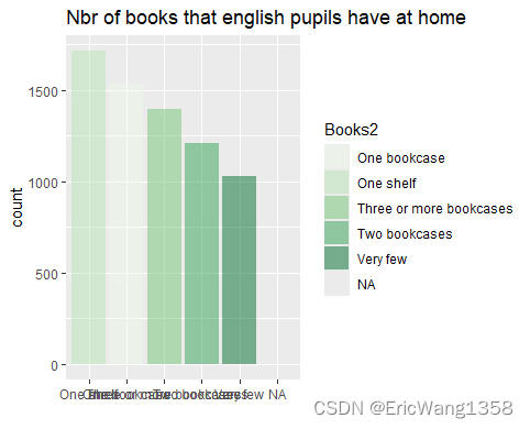
ggplot(smoking_and_drug_use_amongst_English_pupils,aes(fct_infreq(Books2),fill=Books2))+geom_bar(alpha=0.5)+scale_fill_brewer(palette="Greens")+labs(title="Nbr of books that english pupils have at home",x="")
 
#Exercise 3
#3.1
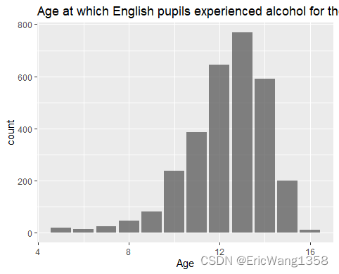
ggplot(smoking_and_drug_use_amongst_English_pupils,aes(x=AlAge2,fill=Sex))+geom_histogram(stat="count", alpha=0.75)+labs(title="Age at which English pupils experienced alcohol for the first time", x="Age")
#3.2
#the distribution is very close for both sex
#3.3
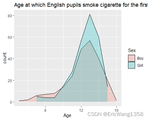
ggplot(smoking_and_drug_use_amongst_English_pupils,aes(x=CgAge2,fill=Sex))+geom_density(stat="count",alpha=0.25)+labs(title="Age at which English pupils smoke cigarette for the first time", x="Age")
 
 

1.1 

1.2

2.1

2.2

2.3

Why the former one don't need fill = Books2 ?

In ggplot2, when you use the fct_infreq() function to reorder a categorical variable like Books2 based on frequency, ggplot automatically creates bars for each level of the reordered variable. This means that each bar in the plot represents a level of the Books2 variable, and the bars are automatically filled based on the default color scheme.

In the second line of code, aes(fct_infreq(Books2), fill=Books2) is used to specify that the fill aesthetic should be mapped to the Books2 variable. This means that the bars in the bar plot will be filled based on the levels of the Books2 variable, and the fct_infreq(Books2) function is used to reorder the bars based on the frequency of each level.

In contrast, in the first line of code, aes(fct_infreq(Books2)) is used without specifying fill=Books2. This means that the bars in the bar plot will be filled with a default color, and the fct_infreq(Books2) function is still used to reorder the bars based on frequency. However, the fill aesthetic is not explicitly mapped to any variable, so the bars will not be filled based on the levels of the Books2 variable and they are the same.

If we delete the fill = part in the 2.3:

ggplot(smoking_and_drug_use_amongst_English_pupils,aes(fct_infreq(Books2)))+geom_bar(alpha=0.5)+scale_fill_brewer(palette="Greens")+labs(title="Nbr of books that english pupils have at home",x="")

The scale_fill_brewer will not work:

3.1

if we delete the fill = sex

3.2