JADE盲分离算法仿真

JADE算法原理

JADE 算法首先通过去均值预白化等预处理过程得到解相关的混合信号，预处理后的信号构建的协方差矩阵变为单位阵，为后续的联合对角化奠定基础；其次，通过建立四阶累积量矩阵，利用高阶累积量的统计独立性等性质从白化后的传感器混合(观测)信号中得到待分解的特征矩阵；最后，通过特征矩阵联合对角化和Givens 旋转得到酉矩阵$U$，从而获得盲源分离算法中混合矩阵$A$ 的有效估计，进而分离出需要的目标信号。
JADE算法的流程图如下：

下面是JADE算法的公式推导，从论文中截的图

JADE仿真程序

JADE算法的函数：

function [A,S]=jade(X,m) 
% Source separation of complex signals with JADE. 
% Jade performs `Source Separation' in the following sense: 
%   X is an n x T data matrix assumed modelled as X = A S + N where 
%  
% o A is an unknown n x m matrix with full rank. 
% o S is a m x T data matrix (source signals) with the properties 
%    	a) for each t, the components of S(:,t) are statistically 
%    	   independent 
% 	b) for each p, the S(p,:) is the realization of a zero-mean 
% 	   `source signal'. 
% 	c) At most one of these processes has a vanishing 4th-order 
% 	   cumulant. 
% o  N is a n x T matrix. It is a realization of a spatially white 
%    Gaussian noise, i.e. Cov(X) = sigma*eye(n) with unknown variance 
%    sigma.  This is probably better than no modeling at all... 
% 
% Jade performs source separation via a  
% Joint Approximate Diagonalization of Eigen-matrices.   
% 
% THIS VERSION ASSUMES ZERO-MEAN SIGNALS 
% 
% Input : 
%   * X: Each column of X is a sample from the n sensors 
%   * m: m is an optional argument for the number of sources. 
%     If ommited, JADE assumes as many sources as sensors. 
% 
% Output : 
%    * A is an n x m estimate of the mixing matrix 
%    * S is an m x T naive (ie pinv(A)*X)  estimate of the source signals 
[n,T]	= size(X); 
 
%%  source detection not implemented yet ! 
if nargin==1, m=n ; end; 
 
 
%%%%%%%%%%%%%%%%%%%%%%%%%%%%%%%%%%%%%%%%%%%%%%%%%%%%%%%%%%%%%%%% 
% A few parameters that could be adjusted 
nem	= m;		% number of eigen-matrices to be diagonalized 
seuil	= 1/sqrt(T)/100;% a statistical threshold for stopping joint diag 
 
 
%%%%%%%%%%%%%%%%%%%%%%%%%%%%%%%%%%%%%%%%%%%%%%%%%%%%%%%%%%%%%%%% 
%%% whitening 
% 
if mseuil, %%% updates matrices M and V by a Givens rotation 
	 	encore 		= 1 ; 
		pair 		= [p;q] ; 
 		G 		= [ c -conj(s) ; s c ] ; 
		V(:,pair) 	= V(:,pair)*G ; 
	 	M(pair,:)	= G' * M(pair,:) ; 
		M(:,[Ip Iq]) 	= [ c*M(:,Ip)+s*M(:,Iq) -conj(s)*M(:,Ip)+c*M(:,Iq) ] ; 
 	end%% if 
  end%% q loop 
 end%% p loop 
end%% while 
 
%%%estimation of the mixing matrix and signal separation 
A	= IW*V; 
S	= V'*Y ; 
 
return ; 
1
2
3
4
5
6
7
8
9
10
11
12
13
14
15
16
17
18
19
20
21
22
23
24
25
26
27
28
29
30
31
32
33
34
35
36
37
38
39
40
41
42
43
44
45
46
47
48
49
50
51
52
53
54
55
56
57
58
59
60
61
62
63
64
65
66
67
68
69
70
71
72
73
74
75
76
77
78
79
80
81
82
83
84
85
86
87
88
89
90
91
92
93
94
95
96
97
98
99
100
101
102
103
104
105
106
107
108
109
110
111
112
113
114
115
116
117
118
119
120
121
122
123
124
125
126
127
128
129
130
131
132
133
134
135
136
137
138
139
140
141
142
143
144
145
146
147
148
149
150
151
152
153
154
155
156
157
158
159
160
161
162
163
164
165
166
167
168
169
170
171
172

主程序：

%% JADE算法仿真
% 输入信号为两段语音，混合矩阵为随机数构成，
% 采用基于四阶累计量的特征矩阵联合近似对角化JADE算法对两段语音进行分离，并绘制了源信号、混合信号和分离信号
% Author:huasir 2023.9.19 Beijing
close all,clear all;clc;
%=========================================================================%
%                          读取语音文件，输入源信号                       %
%=========================================================================%
[S1,fs1] = audioread('E:\sound1.wav'); % 读取原始语音信号，需要将两个语音文件放置在相应目录下
[S2,fs2] = audioread('E:\ICA\sound2.wav');
figure;
subplot(3,2,1),plot(S1),title('输入信号1'); %绘制源信号
subplot(3,2,2),plot(S2),title('输入信号2');
s1 = S1'; %一行代表一个信号
s2 = S2';
S=[s1;s2];  % 将其组成矩阵
%=========================================================================%
%                      对源信号进行混合，得到观测信号                     %
%=========================================================================%
Sweight = rand(size(S,1));  %由随机数构成混合矩阵
MixedS=Sweight*S;     % 将混合矩阵重新排列
subplot(3,2,3),plot(MixedS(1,:)),title('混合信号1'); %绘制混合信号
subplot(3,2,4),plot(MixedS(2,:)),title('混合信号2');
%=========================================================================%
%               采用JADE算法进行盲源分离，得到源信号的估计                %
%=========================================================================%
[Ae,Se]=jade(MixedS,2);  %Ae为估计的混合矩阵，Se为估计的源信号
% 将混合矩阵重新排列并输出
subplot(3,2,5),plot(Se(1,:)),title('JADE解混信号1');
subplot(3,2,6),plot(Se(2,:)),title('JADE解混信号2');
%=========================================================================%
%        源信号、混合信号以及解混合之后的信号的播放                       %
%=========================================================================%
% sound(S1,8000); %播放输入信号1
% sound(S2,8000); %播放输入信号2
% sound(MixedS(1,:),8000); %播放混合信号1
% sound(MixedS(2,:),8000); %播放混合信号2
% sound(Se(1,:),8000); %播放分离信号1
% sound(Se(2,:),8000); %播放分离信号2
fprintf('混合矩阵为：\n'); % 输出混合矩阵以及估计的混合矩阵
disp(Sweight);
fprintf('估计的混合矩阵为：\n');
disp(Ae);
1
2
3
4
5
6
7
8
9
10
11
12
13
14
15
16
17
18
19
20
21
22
23
24
25
26
27
28
29
30
31
32
33
34
35
36
37
38
39
40
41
42
43

然后对其进行混合，混合后调用JADE函数进行解混合，最后对解混合的信号进行绘制并进行读取。
可以听到两段录音的内容不一样，音调也不用，它们满足不相关性，因此能够很好的分离。由下图可以看出，分离后的信号的幅度和真实信号有所不同，并且排序也不同，这是盲分离算法本身的局限性：即幅度模糊性和排序模糊性。但是一般情况下，信号的信息保存在波形的变化中，人们对于其绝对幅度并不敏感。
结果如下图：

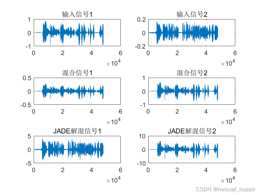
图1. JADE算法分离结果 在主程序中，首先是读取语音文件，语音文件由以下链接给出，当然也可以自己生成源信号。

链接：https://pan.baidu.com/s/1DwnZqDBc1sogERcq7RrVqA
提取码：ngk1