-
Topic 19. 临床预测模型之输出每个患者列线图得分 (nomogramFormula)

点击关注,桓峰基因
临床列线表构建完成,怎么输出列线表每个患者总的得分?
这期就给大家介绍一下,保姆级教程,快来学习吧!
桓峰基因公众号推出基于R语言临床预测模型教程并配有视频在线教程,目前整理出来的教程目录如下:
Topic 10. 单因素 Logistic 回归分析—单因素分析表格
Topic 12 临床预测模型—列线表 (Nomogram)
Topic 13. 临床预测模型—一致性指数 (C-index)
Topic 14. 临床预测模型之校准曲线 (Calibration curve)
Topic 16. 临床预测模型之接收者操作特征曲线 (ROC)
Topic 19. 临床预测模型之输出每个患者列线图得分 (nomogramFormula)
前 言
我们通过Cox回归等方法构建临床预测模型,然后根据模型参数把患者的生存概率可视化为Nomogram。“Nomogra”中文常翻译为诺模图或列线图,其本质就是回归方程的可视化。它根据模型中所有自变量回归系数的大小来制定评分标准,据此给每个自变量的每种取值水平一个评分,这样对每个患者,就可以计算得到一个总分,再通过总分与结局发生概率之间的转换函数来计算每个患者的生存概率。
对于从Nomogram中获得单个患者的得分与相应的生存概率并不困难,但这里有两个技术问题一直困扰着很多研究者:
(1) 如何根据Cox回归列线图精确计算某个患者的风险得分与生存概率?
(2) 如何根据Cox回归列线图精确计算数据集中所有患者得分与生存概率?
实际上,列线图只是Cox回归方程的可视化,无论精确计算单个患者的得分还是预测概率,其依据都是回归方程而非列线图本身。
软件包安装
在输出每个患者总得分,我们需要使用rms软件包构建模型以及绘制列线表,然后进行得分的输出,软件包 nomogramFormula 安装如下:
if(!require(nomogramFormula)) install.packages("nomogramFormula")- 1
- 2
- 3
参数说明
参数有四个,读入预测模型公式,然后选择输出的points是原始数据格式,还是线性预测的结果。
Usage points_cal(formula, rd, lp, digits = 6)
Arguments
formula: the formula of total points with raw data or linear predictors
rd:raw data, which cannot have missing values
lp:linear predictors
digits:default is 6
但是原始数据不能有缺失,有缺失怎么办,看桓峰基因公众号:
例子实操
我们这里举两个例子,一个是软件包 nomogramFormula 自带的例子,另一个我们使用之前讲过Topic 12 临床预测模型—列线表 (Nomogram) 的例子。
例子一
数据读取,如下:
library(rms) # needed for nomogram library(nomogramFormula) set.seed(2018) n <- 2019 age <- rnorm(n, 60, 20) sex <- factor(sample(c("female", "male"), n, TRUE)) sex <- as.numeric(sex) weight <- sample(50:100, n, replace = TRUE) time <- sample(50:800, n, replace = TRUE) units(time) = "day" death <- sample(c(1, 0, 0), n, replace = TRUE) df <- data.frame(time, death, age, sex, weight) head(df) ## time death age sex weight ## 1 55 0 51.54032 1 81 ## 2 770 1 29.00244 1 100 ## 3 685 0 58.71141 2 76 ## 4 78 1 65.41763 1 81 ## 5 340 0 94.70567 1 78 ## 6 54 0 54.70578 1 58 ddist <- datadist(df) oldoption <- options(datadist = "ddist")- 1
- 2
- 3
- 4
- 5
- 6
- 7
- 8
- 9
- 10
- 11
- 12
- 13
- 14
- 15
- 16
- 17
- 18
- 19
- 20
- 21
- 22
- 23
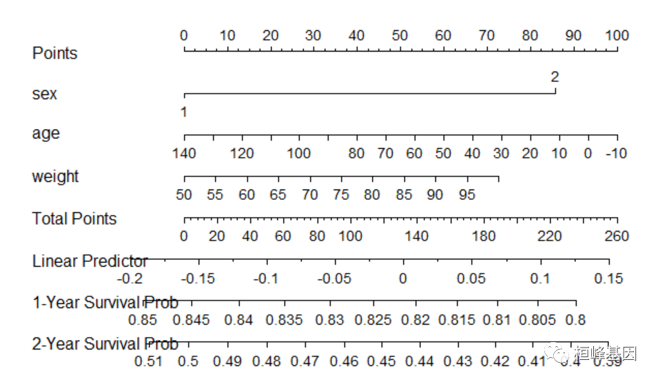
构建模型并绘制列线图:
f <- cph(formula(Surv(time, death) ~ sex + age + weight), data = df, x = TRUE, y = TRUE, surv = TRUE, time.inc = 3) surv <- Survival(f) nomo <- nomogram(f, lp = TRUE, fun = list(function(x) surv(365, x), function(x) surv(365 * 2, x)), funlabel = c("1-Year Survival Prob", "2-Year Survival Prob")) plot(nomo)- 1
- 2
- 3
- 4
- 5
- 6
使用nomogramFormula包中formula_lp()函数及points_cal()函数直接提取训练集中的线性预测值linear.predictors,计算列线图得分,展示前6行。但这种方式仅仅能计算训练集中单个患者的列线图得分。
options(oldoption) # get the formula by the best power using formula_lp results <- formula_lp(nomo) results$formula ## b0 x^1 ## linear predictor 131.9182 821.7001 points <- points_cal(formula = results$formula, lp = f$linear.predictors) head(points) ## 1 2 3 4 5 6 ## 104.02111 146.65643 177.84712 94.76958 70.88473 68.48810- 1
- 2
- 3
- 4
- 5
- 6
- 7
- 8
- 9
- 10
- 11
使用nomogramFormula包中formula_rd()函数及points_cal()函数根据训练集、验证或全集中自变量取值计算列线图得分,并将计算的得分做为新的列添加至对应的数据集中。我们推荐使用这种方法来计算。
# get the formula by the best power using formula_rd results <- formula_rd(nomogram = nomo) results$formula ## b0 x^1 ## sex -85.87254 85.872536 ## age 93.33333 -0.666667 ## weight -72.65806 1.453161 df$points = points_cal(formula = results$formula, rd = df) head(df) ## time death age sex weight points ## 1 55 0 51.54032 1 81 104.02109 ## 2 770 1 29.00244 1 100 146.65641 ## 3 685 0 58.71141 2 76 177.84709 ## 4 78 1 65.41763 1 81 94.76955 ## 5 340 0 94.70567 1 78 70.88469 ## 6 54 0 54.70578 1 58 68.48808- 1
- 2
- 3
- 4
- 5
- 6
- 7
- 8
- 9
- 10
- 11
- 12
- 13
- 14
- 15
- 16
- 17
计算训练集、验证集与全集的线性预测值。训练集的线性预测值从模型cph中直接提取即可,并做为新的列加入到训练集中。
例子二
构建模型并绘制列线图:
library(survival) library(rms) data(package = "survival") lung$sex = factor(lung$sex) lung = na.omit(lung) dd <- datadist(lung) options(datadist = "dd") head(dd) ## $limits ## inst time status age sex ph.ecog ph.karno pat.karno ## Low:effect 3 174.5 1 57.00 70 70 ## Adjust to 11 268.0 1 64.0 1 1 80 80 ## High:effect 15 419.5 2 70.0 1 90 90 ## Low:prediction 1 53.0 1 44.3 1 0 60 60 ## High:prediction 26 737.3 2 75.0 2 2 100 100 ## Low 1 5.0 1 39.0 1 0 50 30 ## High 32 1022.0 2 82.0 2 3 100 100 ## meal.cal wt.loss ## Low:effect 619.0 0.0 ## Adjust to 975.0 7.0 ## High:effect 1162.5 15.0 ## Low:prediction 320.5 -5.0 ## High:prediction 1477.5 35.4 ## Low 96.0 -24.0 ## High 2600.0 68.0 ## ## $values ## $values$status ## [1] 1 2 ## ## $values$sex ## [1] "1" "2" ## ## $values$ph.ecog ## [1] 0 1 2 3 ## ## $values$ph.karno ## [1] 50 60 70 80 90 100 ## ## $values$pat.karno ## [1] 30 40 50 60 70 80 90 100 cph <- cph(Surv(time, status) ~ age + sex + ph.ecog + ph.karno, data = lung, x = TRUE, y = TRUE, surv = TRUE) cph ## Cox Proportional Hazards Model ## ## cph(formula = Surv(time, status) ~ age + sex + ph.ecog + ph.karno, ## data = lung, x = TRUE, y = TRUE, surv = TRUE) ## ## Model Tests Discrimination ## Indexes ## Obs 167 LR chi2 23.46 R2 0.131 ## Events 120 d.f. 4 R2(4,167)0.110 ## Center 2.9977 Pr(> chi2) 0.0001 R2(4,120)0.150 ## Score chi2 23.50 Dxy 0.273 ## Pr(> chi2) 0.0001 ## ## Coef S.E. Wald Z Pr(>|Z|) ## age 0.0129 0.0114 1.13 0.2586 ## sex=2 -0.5239 0.1978 -2.65 0.0081 ## ph.ecog 0.7426 0.2086 3.56 0.0004 ## ph.karno 0.0205 0.0113 1.81 0.0699 ## survival <- Survival(cph) survival1 <- function(x) survival(365, x) survival2 <- function(x) survival(730, x) nom <- nomogram(cph, fun = list(survival1, survival2), fun.at = c(0.05, seq(0.1, 0.9, by = 0.05), 0.95), funlabel = c("1 year survival", "2 year survival")) plot(nom) - 1
- 2
- 3
- 4
- 5
- 6
- 7
- 8
- 9
- 10
- 11
- 12
- 13
- 14
- 15
- 16
- 17
- 18
- 19
- 20
- 21
- 22
- 23
- 24
- 25
- 26
- 27
- 28
- 29
- 30
- 31
- 32
- 33
- 34
- 35
- 36
- 37
- 38
- 39
- 40
- 41
- 42
- 43
- 44
- 45
- 46
- 47
- 48
- 49
- 50
- 51
- 52
- 53
- 54
- 55
- 56
- 57
- 58
- 59
- 60
- 61
- 62
- 63
- 64
- 65
- 66
- 67
- 68
- 69
- 70

计算每个患者的总得分:
# get the formula by the best power using formula_lp results <- formula_lp(nom) points <- points_cal(formula = results$formula, lp = cph$linear.predictors) head(points) ## 1 2 3 4 5 6 ## 79.39907 106.36008 79.44563 104.16493 96.71219 85.66158 # get the formula by the best power using formula_rd results <- formula_rd(nomogram = nom) lung$points <- points_cal(formula = results$formula, rd = lung) head(lung) ## inst time status age sex ph.ecog ph.karno pat.karno meal.cal wt.loss ## 2 3 455 2 68 1 0 90 90 1225 15 ## 4 5 210 2 57 1 1 90 60 1150 11 ## 6 12 1022 1 74 1 1 50 80 513 0 ## 7 7 310 2 68 2 2 70 60 384 10 ## 8 11 361 2 71 2 2 60 80 538 1 ## 9 1 218 2 53 1 1 70 80 825 16 ## points ## 2 79.39909 ## 4 106.36010 ## 6 79.44564 ## 7 104.16495 ## 8 96.71220 ## 9 85.66160- 1
- 2
- 3
- 4
- 5
- 6
- 7
- 8
- 9
- 10
- 11
- 12
- 13
- 14
- 15
- 16
- 17
- 18
- 19
- 20
- 21
- 22
- 23
- 24
- 25
整个过程是不是非常简单好用?学会了都是自己的本事,想学更多本领快来关注桓峰基因公众号,更多的免费文字版教程结合视频版教程相结合,保证您来了就有收获!!!
桓峰基因,铸造成功的您!
有想进生信交流群的老师可以扫最后一个二维码加微信,备注“单位+姓名+目的”,有些想发广告的就免打扰吧,还得费力气把你踢出去!
References:
- nomogramFormula: Calculate Total Points and Probabilities for Nomogram. Version: 1.2.0.0

-
相关阅读:
前端面试题日常练-day45 【面试题】
UiPath实战(08) - 选取器(Selector)
用核心AI资产打造稀缺电竞体验,顺网灵悉背后有一盘大棋
管程的定义以及基本特征
【毕业设计】基于Django与深度学习的股票预测系统
工业机器人常用的六种坐标系
NoSQL
通过jsoup抓取谷歌商店评分
TestDeploy v3.0构思
华为机试题解析020:数据分类处理(python)
- 原文地址:https://blog.csdn.net/weixin_41368414/article/details/127317049
