《Python 计算机视觉编程》学习笔记（三）

第3章图像到图像的映射

引言

本章讲解图像之间的变换，以及一些计算变换的实用方法。这些变换可以用于图像扭曲变形和图像配准。

3.1 单应性变换

单应性变换是将一个平面内的点映射到另一个平面内的二维投影变换。在这里，平面是指图像或者三维中的平面表面。本质上，单应性变换 H，按照下面的方程映射二维中的点（齐次坐标意义下）：
$\left[x′y′w′$

x' y' w'

\right]=\left[

h 1 h 4 h 7 h 2 h 5 h 8 h 3 h 6 h 9

\right]\left[

x y w

\right] 或 \mathbf{x}^{\prime}=\boldsymbol{H} \mathbf{x}

⎣ ⎡ x^{'} y^{'} w^{'} ⎦ ⎤ = ⎣ ⎡ h_{1} h_{4} h_{7} h_{2} h_{5} h_{8} h_{3} h_{6} h_{9} ⎦ ⎤ ⎣ ⎡ x y w ⎦ ⎤ 或 x^{'} = H x

点的齐次坐标是依赖于其尺度定义的，所以， $x = [x, y, w] = [αx, α y, α w] = [x / w, y / w, 1]$ 都表示同一个二维点。因此，单应性矩阵 H 也仅依赖尺度定义，所以，单应性矩阵具有 8 个独立的自由度。我们通常使用 w=1 来归一化点，这样，点具有唯一的图像坐标 x 和 y。这个额外的坐标使得我们可以简单地使用一个矩阵来表示变换。

相似变换：

$\left[x′y′1$

x' y' 1

\right]=\left[

s cos (θ) s sin (θ) 0 - s sin (θ) s cos (θ) 0 t x t y 1

\right]\left[

x y 1

\right] \quad \text { 或 } \quad \boldsymbol{x}^{\prime}=\left[

\right] \boldsymbol{x}

⎣ ⎡ x^{'} y^{'} 1 ⎦ ⎤ = ⎣ ⎡ s cos (θ) s sin (θ) 0 - s sin (θ) s cos (θ) 0 t_{x} t_{y} 1 ⎦ ⎤ ⎣ ⎡ x y 1 ⎦ ⎤ 或 x^{'} = [s R 0 t 1] x

是一个包含尺度变化的二维刚体变换。上式中的向量 s 指定了变换的尺度，R 是角度为 θ 的旋转矩阵， $t=[t_x ,t_y ]$ 在这里也是一个平移向量。如果 s=1，那么该变换能够保持距离不变。此时，变换为刚体变换。相似变换可以用于很多应用，比如图像配准。

3.1.1　直接线性变换算法

单应性矩阵可以由两幅图像（或者平面）中对应点对计算出来。一个完全射影变换具有 8 个自由度。根据对应点约束，每个对应点对可以写出两个方程，分别对应于 x 和 y 坐标。因此，计算单应性矩阵 H 需要４个对应点对。DLT（Direct Linear Transformation，直接线性变换）是给定４个或者更多对应点对矩阵，来计算单应性矩阵 H 的算法。

将单应性矩阵 H 作用在对应点对上，重新写出该方程，我们可以得到下面的方程：
$\left[−x1−y1−1000x1x′1y1x′1x′1000−x1−y1−1x1y′1y1y′1y′1−x2−y2−1000x2x′2y2x′2x′2000−x2−y2−1x2y′2y2y′2y′2⋮⋮⋮⋮$

\right]\left[

\right]=\mathbf{0}或者 Ah=0

⎣ ⎡ - x_{1} 0 - x_{2} 0 - y_{1} 0 - y_{2} 0 ⋮ - 1 0 - 1 0 0 - x_{1} 0 - x_{2} ⋮ 0 - y_{1} 0 - y_{2} 0 - 1 0 - 1 ⋮ x_{1} x_{1}^{'} x_{1} y_{1}^{'} x_{2} x_{2}^{'} x_{2} y_{2}^{'} y_{1} x_{1}^{'} y_{1} y_{1}^{'} y_{2} x_{2}^{'} y_{2} y_{2}^{'} ⋮ x_{1}^{'} y_{1}^{'} x_{2}^{'} y_{2}^{'} ⎦ ⎤ ⎣ ⎡ h_{1} h_{2} h_{3} h_{4} h_{5} h_{6} h_{7} h_{8} h_{9} ⎦ ⎤ = 0 或者 A h = 0

其中 A 是一个具有对应点对二倍数量行数的矩阵。将这些对应点对方程的系数堆叠到一个矩阵中，我们可以使用 SVD（Singular Value Decomposition，奇异值分解）算法找到 H 的最小二乘解。

3.1.2　仿射变换

$\left[x′y′1$

\right]=\left[

\right]\left[

\right] \quad \text { 或 } \quad \boldsymbol{x}^{\prime}=\left[

\right] \boldsymbol{x}

⎣ ⎡ x^{'} y^{'} 1 ⎦ ⎤ = ⎣ ⎡ a_{1} a_{3} 0 a_{2} a_{4} 0 t_{x} t_{y} 1 ⎦ ⎤ ⎣ ⎡ x y 1 ⎦ ⎤ 或 x^{'} = [A 0 t 1] x

保持了 w=1, 不具有投影变换所具有的强大变形能力。仿射变换包含一个可逆矩阵 A 和一个平移向量 $t=[t_x ,t_y ]$ 。仿射变换可以用于很多应用，比如图像扭曲。

仿射变换具有 6 个自由度，因此我们需要三个对应点对来估计矩阵 H。通过将最后两个元素设置为 0，即 $h_7 =h_8 =0$ ，仿射变换可以用上面的 DLT 算法估计得出。

3.2　图像扭曲

对图像块应用仿射变换，我们将其称为图像扭曲（或者仿射扭曲）。

from fileinput import filename
from scipy import ndimage
from PIL import Image
from numpy import * 
from pylab import *
import time



def imageTransform(imgpath):
    """  
        函数功能：扭曲输入的图片 
        参数说明：imgpath__图像数据路径
        函数返回：无
    """
    img = array(Image.open(imgpath[0]).convert('L'))
    gray()
    H = array([[1.4, 0.05, -100], [0.05, 1.5, -100], [0, 0, 1]])
    # 扭曲操作 ndimage.affine_transform(im,A,b,size)
    # 线性变换 A 和一个平移向量 b 来对图像块应用仿射变换。
    # 选项参数 size 可以用来指定输出图像的大小。
    # 默认输出图像设置为和原始图像同样大小。
    img_re = ndimage.affine_transform(img, H[:2, :2], (H[0, 2], H[1, 2]))

    subplot(121)
    imshow(img), title('original')
    subplot(122)
    imshow(img_re), title('result')
    # savefig('image.jpg', dpi=600,bbox_inches='tight')
    # dpi：分辨率，默认100
    # bbox_inches： 要保存的图片范围。‘tight’表示去掉周边空白。
    savefig('figure/testblueline.jpg',dpi=600,bbox_inches='tight')
    show()

    return
	
def main():

    imagepath = [r"C:/hqq/document/python/computervision/ch03/figure/picture1.jpg",
                 r"C:/hqq/document/python/computervision/ch03/figure/picture2.jpg"]

    imageTransform(imagepath)

    return

if __name__ == '__main__':
    
    timeStart = time.time()
    main()
    timeEnd = time.time()
    print("the program running time is :",timeEnd-timeStart)

输出图像如下：
在这里插入图片描述
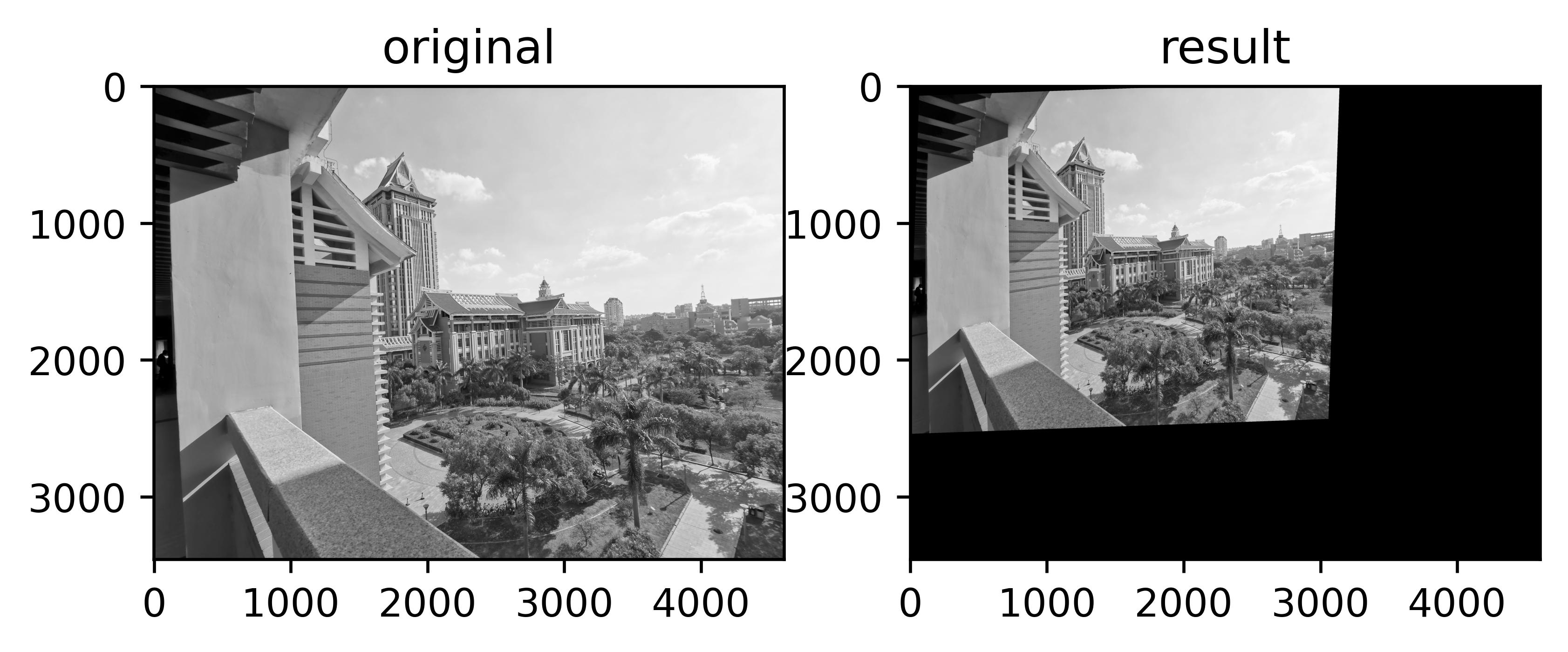
右图为扭曲后的图片，大小和图片形状都发生了改变。

3.2.1　图像中的图像

射扭曲的一个简单例子是，将图像或者图像的一部分放置在另一幅图像中，使得它们能够和指定的区域或者标记物对齐。


def Haffine_from_points(fp, tp):
    """
    计算H，仿射变换，使得tp是fp经过仿射变换H得到的
    :param fp: 
    :param tp: 
    :return: 
    """
    if fp.shape != tp.shape:
        raise RuntimeError('number of points do not match')
    
    # 对点进行归一化
    # --映射起始点--
    m = mean(fp[:2], axis=1)
    maxstd = max(std(fp[:2], axis=1)) + 1e-9
    C1 = diag([1/maxstd, 1/maxstd, 1])
    C1[0][2] = -m[0]/maxstd
    C1[1][2] = -m[1]/maxstd
    fp_cond = dot(C1, fp)
    # 映射对应点
    m = mean(tp[:2], axis=1)
    maxstd = max(std(tp[:2], axis=1)) + 1e-9
    C2 = diag([1/maxstd, 1/maxstd, 1])
    C2[0][2] = -m[0]/maxstd
    C2[1][2] = -m[1]/maxstd
    tp_cond = dot(C2, tp)
    
    # 因为归一化后的点均值为0，故平移量为0
    A = concatenate((fp_cond[:2], tp_cond[:2]), axis=0)
    U, S, V = linalg.svd(A.T)
    
    # 创建矩阵B,C
    temp = V[:2].T
    B = temp[:2]
    C = temp[2:4]
    temp2 = concatenate((dot(C, linalg.pinv(B)), zeros((2, 1))), axis=1)
    H = vstack((temp2, [0, 0, 1]))
    
    # 反归一化
    H = dot(linalg.inv(C2), dot(H,C1))
    return H / H[2, 2]

def warp_image_in_image(im1,im2,tp):
    """ Put im1 in im2 with an affine transformation
        such that corners are as close to tp as possible.
        tp are homogeneous and counter-clockwise from top left. """ 
    
    # points to warp from
    m,n = im1.shape[:2]
    fp = array([[0,m,m,0],[0,0,n,n],[1,1,1,1]])
    
    # compute affine transform and apply
    H = Haffine_from_points(tp,fp)
    im1_t = ndimage.affine_transform(im1,H[:2,:2],
                    (H[0,2],H[1,2]),im2.shape[:2])
    alpha = (im1_t > 0)
    
    return (1-alpha)*im2 + alpha*im1_t

def image_in_image(imagepath):
    """  
        函数功能：将一幅图片加到另一幅图片中
        参数说明：imgpath__图像数据路径
        函数返回：无
    """
    img1 = array(Image.open(imagepath[6]).convert('L'))
    img2 = array(Image.open(imagepath[7]).convert('L'))
    gray()
    # 选定一些目标点
    # [264, 538, 540, 264], [40, 36, 605, 605]
    # 这两组数据对应图像上的四个点，顺序是从左上角开始，逆时针旋转。
    tp1 = array([[264, 538, 540, 264], [40, 36, 605, 605], [1, 1, 1, 1]])
    tp2 = array([[264,538,250,264],[40,63,605,300],[1,1,1,1]])
    
    # 这里选择两张图片要替换的位置前四个选择的点与后四个选择的点
    imshow(img1)
    x = ginput(8)
    print("you click:", x)
    matData = mat(x)
    axis_x = matData[:,1]
    axis_y = matData[:,0]
    print('axis_x:',axis_x)
    print('axis_y:',axis_y)
    for i in range(4):
        tp1[0][i] = axis_x[i]
        tp1[1][i] = axis_y[i]
        # print('asis_x:',axis_x[i])
    print('tp1:',tp1)
    for j in range(4):
        tp2[0][j] = axis_x[j+4]
        tp2[1][j] = axis_y[j+4]
        # print('asis_x: i:',axis_x[i],i)
    print('tp2:',tp2)
    # img3 = warp.image_in_image(img2, img1, tp1)
    # img4 = warp.image_in_image(img2, img1, tp2)
    
    #把warp中的函数复制过来了
    img3 = warp_image_in_image(img2, img1, tp1)
    img4 = warp_image_in_image(img2, img1, tp2)
    
    subplot(221)
    imshow(img1), title('original1'), axis('off')
    subplot(222)
    imshow(img2), title('original2'), axis('off')
    subplot(223)
    imshow(img3), title('tp1_result'), axis('off')
    subplot(224)
    imshow(img4), title('tp2_result'), axis('off')

    savefig('testout/test2.jpg',dpi=600,bbox_inches='tight')
    show()

    return

'运行

输出如下：
在这里插入图片描述
点选了需要替换的位置后，程序就会将图像1的对应部分用图像2给替换掉。

将扭曲的图像和第二幅图像融合，我们就创建了 alpha 图像。该图像定义了每个像素从各个图像中获取的像素值成分多少。这里我们基于以下事实，扭曲的图像是在扭曲区域边界之外以 0 来填充的图像，来创建一个二值的 alpha 图像。严格意义上说，我们需要在第一幅图像中的潜在 0 像素上加上一个小的数值，或者合理地处理这些 0 像素。

3.2.2　分段仿射扭曲

三角形图像块的仿射扭曲可以完成角点的精确匹配。

对应点对集合之间最常用的扭曲方式：分段仿射扭曲。

给定任意图像的标记点，通过将这些点进行三角剖分，然后使用仿射扭曲来扭曲每个三角形，我们可以将图像和另一幅图像的对应标记点扭曲对应。为了三角化这些点，我们经常使用狄洛克三角剖分方法。

下面程序实现随机点三角化。


from scipy.spatial import Delaunay
from numpy import *

def triangulatePoints():
    """  
        函数功能：将随机点三角化
        参数说明：无
        函数返回：无
    """
    # 生成随机点
    x, y = array(random.standard_normal((2, 100)))
    tri = Delaunay(np.c_[x, y]).simplices
    figure()
    subplot(121)
    for t in tri:
        # 将第一个点加入到最后
        t_ext = [t[0], t[1], t[2], t[0]] 
        plot(x[t_ext], y[t_ext], 'r')
    plot(x, y, '*'), axis('off'),title("随机点三角化",fontproperties = myfont)
    
    subplot(122)
    plot(x, y, '*'),axis('off'),title("随机点",fontproperties = myfont)
    savefig('testout/test3.jpg',dpi =600,bbox_inches='tight')
    show()
    
    return

输出结果如下：
在这里插入图片描述

彩色图像分段扭曲仿射

代码如下：


def triangulatePoints():
    """  
        函数功能：将随机点三角化
        参数说明：无
        函数返回：无
    """
    # 生成随机点
    x, y = array(random.standard_normal((2, 100)))
    tri = Delaunay(np.c_[x, y]).simplices
    figure()
    subplot(121)
    for t in tri:
        # 将第一个点加入到最后
        t_ext = [t[0], t[1], t[2], t[0]] 
        plot(x[t_ext], y[t_ext], 'r')
    plot(x, y, '*'), axis('off'),title("随机点三角化",fontproperties = myfont)
    
    subplot(122)
    plot(x, y, '*'),axis('off'),title("随机点",fontproperties = myfont)
    savefig('testout/test3.jpg',dpi =600,bbox_inches='tight')
    show()
    
    return

def alpha_for_triangle(points,m,n):
    """ 对于带有由 points 定义角点的三角形，创建大小为 (m, n) 的 alpha 图  
        (在归一化的齐次坐标意义下） 
    """
    alpha = zeros((m,n))
    for i in range(int(min(points[0])),int(max(points[0]))):
        for j in range(int(min(points[1])),int(max(points[1]))):
            x = linalg.solve(points, [i, j, 1])
            if min(x) > 0: # 所有系数都大于零
                alpha[i,j] = 1
    return alpha


def pw_affine(fromim,toim,fp,tp,tri):
    """ 从一幅图像中扭曲矩形图像块
    fromim= 将要扭曲的图像
    toim= 目标图像
    fp= 齐次坐标表示下，扭曲前的点
    tp= 齐次坐标表示下，扭曲后的点
    tri= 三角剖分 """
    im = toim.copy()
    # 检查图像是灰度图像还是彩色图象
    is_color = len(fromim.shape) == 3
    # 创建扭曲后的图像（如果需要对彩色图像的每个颜色通道进行迭代操作，那么有必要这样做）
    im_t = zeros(im.shape, 'uint8')
    for t in tri:
        # 计算仿射变换
        #tp的第t[0]行、tp的第t[1]行、tp的第t[2]行、
        H = Haffine_from_points(tp[:,t],fp[:,t])
        if is_color:
            for col in range(3):
                im_t[:,:,col] = ndimage.affine_transform(fromim[:,:,col],H[:2,:2],(H[0,2],H[1,2]),im.shape[:2])
        else:
            im_t = ndimage.affine_transform(fromim,H[:2,:2],(H[0,2],H[1,2]),im.shape[:2])
        # 三角形的 alpha
        alpha = alpha_for_triangle(tp[:,t],im.shape[0],im.shape[1])
        # 将三角形加入到图像中
        im[alpha>0] = im_t[alpha>0]
    return im

def plot_mesh(x,y,tri):
    """ 绘制三角形 """
    for t in tri:
        t_ext = [t[0], t[1], t[2], t[0]]  # 将第一个点加入到最后
        plot(x[t_ext], y[t_ext], 'r')
    
    return

def affineColorFigure(figurepath):
    """  
        函数功能：彩色图像扭曲
        参数说明：无
        函数返回：无
    """
    # # 打开图像，并将其扭曲
    # img1 = array(Image.open(figurepath[7]))
    # imshow(img1)
    # x = ginput(30)
    # print("you click:", x)
    # savetxt('data.txt',x)

    # 这里要注意选择的图片大小，应该是一个大一个小，我们再小的上选点，将大的扭曲过来
    fromim = array(Image.open(figurepath[6]))

    x, y = meshgrid(range(5), range(6))
    
    x = (fromim.shape[1]/4) * x.flatten()
    y = (fromim.shape[0]/5) * y.flatten()
    # 三角剖分
    tri = Delaunay(np.c_[x, y]).simplices 
    # 打开图像和目标点
    im = array(Image.open(figurepath[5]))
    # tp = loadtxt('data.txt')  # destination points
    tp = loadtxt('turningtorso1_points.txt')  # destination points
    
    # 将点转换成齐次坐标
    fp = vstack((y, x, ones((1, len(x)))))
    tp = vstack((tp[:, 1], tp[:, 0], ones((1, len(tp)))))
    # 扭曲三角形
    im = pw_affine(fromim, im, fp, tp, tri)


    # 绘制图像
    figure()
    imshow(im)
    plot_mesh(tp[1], tp[0], tri),axis('off')
    savefig('testout/test3.jpg',dpi =600,bbox_inches='tight')
    show()
    
    return
'运行

输出图片如下：
在这里插入图片描述
注意一点过要选择合适大小的图片，否则程序会报错，所以记得要一张大一点的图片和一张小一点的图片，如果报错，就交换一下。还有图片差异不能太大，否则扭曲过来的效果就会很差。当然还有个问题是点的选择，我选的点出来的效果不如书中给的点的。不知道问题在哪。

3.2.3　图像配准

图像配准是对图像进行变换，使变换后的图像能够在常见的坐标系中对齐。配准可以是严格配准，也可以是非严格配准。为了能够进行图像对比和更精细的图像分析，图像配准是一步非常重要的操作。

多个人脸图像进行严格配准类型的配准中，我们实际上是寻找一个相似变换（带有尺度变化的刚体变换），在对应点对之间建立映射。

使用未准确配准的图像同样对主成分的计算结果有着很大的影响。

配准算法的一般步骤：

特征提取
特征匹配
估计变换模型
图像重采样及变换

特征提取

特征提取是指分别提取两幅图像中共有的图像特征，这种特征是出现在两幅图像中对比列、旋转、平移等变换保持一致性的特征，如线交叉点、物体边缘角点、虚圆闭区域的中心等可提取的特征。特征包括：点、线和面三类。

点特征包括下面几种算法： Harris算法、Susan算法、 Harris-Laplace算法、SIFT特征点提取、SURF特征点提取

线特征是图像中明显的线段特征，如道路河流的边缘，目标的轮廓线等。线特征的提取一般分两步进行：首先采用某种算法提取出图像中明显的线段信息，然后利用限制条件筛选出满足条件的线段作为线特征。

面特征是指利用图像中明显的区域信息作为特征。在实际的应用中最后可能也是利用区域的重心或圆的圆心点等作为特征。

这段看的是师姐的博客——>python计算机视觉编程写的特别详细，大家想进一步了解可以看一下。

特征匹配

特征匹配分两步
a. 对特征作描述
现有的主要特征描述子：SIFT特征描述子，SURF特征描述子，对比度直方图（CCH）,DAISY特征描述子，矩方法。
b. 利用相似度准则进行特征匹配
常用的相似性测度准则有如欧式距离，马氏距离，Hausdorff距离等。

估计变换模型

空间变换模型是所有配准技术中需要考虑的一个重要因素，各种配准技术都要建立自己的变换模型，变换空间的选取与图像的变形特性有关。常用的空间变换模型有：刚体变换、仿射变换、投影变换、非线性变换。

图像重采样及变换

在得到两幅图像的变换参数后，要将输入图像做相应参数的变换，使之与参考图像处于同一坐标系下，则矫正后的输入图像与参考图像可用作后续的图像融合、目标变化检测处理或图像镶嵌；
涉及输入图像变换后所得点坐标不一定为整像素数，则应进行插值处理。常用的插值算法有最近领域法，双线性插值法和立方卷积插值法

3.3　创建全景图

在同一位置（即图像的照相机位置相同）拍摄的两幅或者多幅图像是单应性相关的。我们经常使用该约束将很多图像缝补起来，拼成一个大的图像来创建全景图像。
创建全景图像步骤大致分为以下几点：

创建全景图像步骤大致分为以下几点：

图片之间：

特征点匹配：找到素材图片中共有的图像部分。
图片匹配：连接匹配的特征点，估算图像间几何方面的变换。

全局优化和无缝衔接：

全景图矫直：矫正拍摄图片时相机的相对3D旋转，主要原因是拍摄图片时相机很可能并不在同一水平线上，并且存在不同程度的倾斜，略过这一步可能导致全景图变成波浪形状。
图像均衡补偿：全局平衡所有图片的光照和色调。
图像频段融合：步骤4之后仍然会存在图像之间衔接边缘、晕影效果（图像的外围部分的亮度或饱和度比中心区域低）、视差效果（因为相机透镜移动导致）。

RANSAC（RANdom SAmple Consensus 随机一致性采样）

该方法是用来找到正确模型来拟合带有噪声数据的迭代方法。给定一个模型，例如点集之间的单应性矩阵， RANSAC 基本的思想是，数据中包含正确的点和噪声点，合理的模型应该能够在描述正确数据点的同时摒弃噪声点。

RANSAC 的标准例子：用一条直线拟合带有噪声数据的点集。简单的最小二乘在该例子中可能会失效，但是 RANSAC 能够挑选出正确的点，然后获取能够正确拟合的直线。

连续图像对间匹配对应点对

在连续图像对间使用 SIFT 特征寻找匹配对应点对。程序实现如下：


def findHomographyMatrix(imagepath):
    # 提取特征并匹配使用sift算法
    
    # 批量修改图像尺寸
    for maindir, subdir,file_name_list in os.walk(imagepath):
        print(file_name_list)
        for file_name in file_name_list:
            if file_name[:-3] == 'jpg':
                image=os.path.join(maindir,file_name) #获取每张图片的路径
                file=Image.open(image)
                out=file.resize((1000,900),Image.Resampling.LANCZOS)  #以高质量修改图片尺寸为（1000.900）
                out.save(image)                            #以同名保存到原路径

    # 设置数据文件夹的路径
    featname = [imagepath +'/' + str(i + 1) + '.sift' for i in range(5)]
    imname = [imagepath + '/picture' + str(i + 1) + '.jpg' for i in range(5)]

    l = {}
    d = {}
    for i in range(5):
        harris.process_image(imname[i], featname[i])
        l[i], d[i] = harris.read_features_from_file(featname[i])

    matches = {}
    for i in range(4):
        matches[i] = harris.match(d[i + 1], d[i])

    # 可视化匹配
    for i in range(4):
        im1 = array(Image.open(imname[i]))
        im2 = array(Image.open(imname[i + 1]))
        plt.figure()
        harris.plot_matches(im2, im1, l[i + 1], l[i], matches[i], show_below=True)
    
    show()
    return
'运行

输出如下：
在这里插入图片描述

显然，并不是所有图像中的对应点对都是正确的。实际上， SIFT 是具有很强稳健性的描述子，能够比其他描述子，例如图像块相关的 Harris 角点，产生更少的错误的匹配。

3.3.3　拼接图像


def panorama(H,fromim,toim,padding=2400,delta=2400):
    """ 使用单应性矩阵 H(使用 RANSAC 健壮性估计得出)，协调两幅图像，创建水平全景图像。结果
    为一幅和 toim 具有相同高度的图像。 padding 指定填充像素的数目， delta 指定额外的平移量 
    """
    # 检查图像是灰度图像，还是彩色图像
    is_color = len(fromim.shape) == 3
    # 用于 geometric_transform() 的单应性变换
    def transf(p):
        p2 = dot(H,[p[0],p[1],1])
        return (p2[0]/p2[2],p2[1]/p2[2])
    if H[1,2]<0: # fromim 在右边
        print ('warp - right')
        # 变换 fromim
        if is_color:
            # 在目标图像的右边填充 0
            toim_t = hstack((toim,zeros((toim.shape[0],padding,3))))
            fromim_t = zeros((toim.shape[0],toim.shape[1]+padding,toim.shape[2]))
            for col in range(3):
                fromim_t[:, :, col] = ndimage.geometric_transform(
                    fromim[:, :, col], transf, (toim.shape[0], toim.shape[1]+padding))
        else:
            # 在目标图像的右边填充 0
            toim_t = hstack((toim,zeros((toim.shape[0],padding))))
            fromim_t = ndimage.geometric_transform(fromim, transf,
                                                (toim.shape[0], toim.shape[1]+padding))
    else:
        print ('warp - left')
        # 为了补偿填充效果，在左边加入平移量
        H_delta = array([[1,0,0],[0,1,-delta],[0,0,1]])
        H = dot(H,H_delta)
        # fromim 变换
        if is_color:
        # 在目标图像的左边填充 0
            toim_t = hstack((zeros((toim.shape[0],padding,3)),toim))
            fromim_t = zeros((toim.shape[0],toim.shape[1]+padding,toim.shape[2]))
            for col in range(3):
                fromim_t[:, :, col] = ndimage.geometric_transform(fromim[:, :, col],
                                                                  transf, (toim.shape[0], toim.shape[1]+padding))
        else:
            # 在目标图像的左边填充 0
            toim_t = hstack((zeros((toim.shape[0],padding)),toim))
            fromim_t = ndimage.geometric_transform(fromim,transf,(toim.shape[0],toim.shape[1]+padding))
    # 协调后返回（将 fromim 放置在 toim 上）
    if is_color:
        # 所有非黑色像素
        alpha = ((fromim_t[:,:,0] * fromim_t[:,:,1] * fromim_t[:,:,2] ) > 0)
        for col in range(3):
            toim_t[:,:,col] = fromim_t[:,:,col]*alpha + toim_t[:,:,col]*(1-alpha)
    else:
        alpha = (fromim_t > 0)
        toim_t = fromim_t*alpha + toim_t*(1-alpha)
    return toim_t


def H_from_ransac(fp,tp,model,maxiter=1000,match_theshold=10):
    """ 使用 RANSAC 稳健性估计点对应间的单应性矩阵 H(ransac.py 为从
    http://www.scipy.org/Cookbook/RANSAC 下载的版本）
    # 输入：齐次坐标表示的点 fp, tp(3 x n 的数组） 
    """
    import ransac
    # 对应点组
    data = vstack((fp, tp))
    # 计算 H，并返回
    H, ransac_data = ransac.ransac(
        data.T, model, 4, maxiter, match_theshold, 10, return_all=True)
    return H, ransac_data['inliers']


def make_homog(points):
    """ Convert a set of points (dim*n array) to 
        homogeneous coordinates. """
        
    return vstack((points,ones((1,points.shape[1])))) 
 

# 将匹配转换成齐次坐标点的函数
def convert_points(matches,j,l):
    ndx = matches[j].nonzero()[0]
    fp = make_homog(l[j + 1][ndx, :2].T)
    ndx2 = [int(matches[j][i]) for i in ndx]
    tp = make_homog(l[j][ndx2, :2].T)

    # switch x and y - TODO this should move elsewhere
    fp = vstack([fp[1], fp[0], fp[2]])
    tp = vstack([tp[1], tp[0], tp[2]])
    return fp, tp


def stitchImage(matches,imname,l):
    # 估计单应性矩阵
    model = homography.RansacModel()

    fp, tp = convert_points(matches,1,l)
    H_12 = H_from_ransac(fp, tp, model)[0]  # im1 到im2 的单应性矩阵

    fp, tp = convert_points(matches,0,l)
    H_01 = H_from_ransac(fp, tp, model)[0]  # im0 到im1 的单应性矩阵

    tp, fp = convert_points(matches,2,l)  # 注意：点是反序的
    H_32 = H_from_ransac(fp, tp, model)[0]  # im3 到im2 的单应性矩阵

    tp, fp = convert_points(matches,3,l)  # 注意：点是反序的
    H_43 = H_from_ransac(fp, tp, model)[0]  # im4 到im3 的单应性矩阵

    # 扭曲图像
    delta = 2000  # 用于填充和平移

    im1 = array(Image.open(imname[1]), "uint8")
    im2 = array(Image.open(imname[2]), "uint8")
    im_12 = panorama(H_12, im1, im2, delta, delta)

    im1 = array(Image.open(imname[0]), "f")
    im_02 = panorama(dot(H_12, H_01), im1, im_12, delta, delta)

    im1 = array(Image.open(imname[3]), "f")
    im_32 = panorama(H_32, im1, im_02, delta, delta)

    im1 = array(Image.open(imname[4]), "f")
    im_42 = panorama(dot(H_32, H_43), im1, im_32, delta, 2 * delta)

    plt.figure()
    plt.imshow(array(im_42, "uint8"))
    plt.axis('off')
    plt.show()

    return

'运行

输出结果如下：

在这里插入图片描述
这是第一次输出的，图片顺寻序不对，导致输出的完全变形了。
给图片重新排了序（换了图库）输出如下：

在这里插入图片描述

这是用的别的图库抛出的结果，对比图库我发现我的库中的图片变化太大，就是转的角度太大，而这个库的图片变化的并不大，转角较小或许这是一个原因。（转角小所以匹配点多，所以容易拼接？）所以我输出的就不对。后面有时间可以再换个图像跑一下。

3.4小结

本章主要的是单应性变换，将一个投影平面的点通过乘以一个变换矩阵转换到另外一个平面。我理解的是两幅图片作比较不太容易进行，所以我们找到两个图像的共同点（看了点别的资料，此处给出单应性不严谨的定义：用 [无镜头畸变] 的相机从不同位置拍摄 [同一平面物体] 的图像之间存在单应性，可以用 [投影变换] 表示。来自知乎单应性Homograph估计：从传统算法到深度学习），通过乘一个矩阵，就可以将两幅图像转到一个平面，便于进行操作处理。感觉我们做的就是把图像存到矩阵或数组中，然后使用数学概念把这些矩阵颠来倒去，翻来覆去的折腾，当然这些操作都有理论支撑的，并不是儿戏。突然觉得不应该叫图像处理，应该叫矩阵基本运算及其实际应用。

本章代码实现的不怎么样，也没有全部跑一下，贴出来仅供大家参考。

链接：https://pan.baidu.com/s/1UlhGm_JfjYMolUCnzWtkew?pwd=ptvw
提取码：ptvw

有需要自取。

相关阅读:
防火墙基础实验配置
分布式事务之Seata介绍
力扣labuladong一刷day2共7题
C语言三大结构
艾美捷A型CpG DNA, 人/小鼠应用和化学性质说明
【测试沉思录】16. 性能测试中的系统资源分析之三：磁盘
FRED案例：矩形微透镜阵列
Java输入/输出之RandomAccessFile的功能和用法
QT day3
Graph Self-Supervised Learning: A Survey

原文地址：https://blog.csdn.net/qq_35021992/article/details/127061042

《Python 计算机视觉编程》学习笔记（三）

文章目录

第3章 图像到图像的映射

引言

3.1 单应性变换

相似变换：

3.1.1 直接线性变换算法

3.1.2 仿射变换

3.2 图像扭曲

3.2.1 图像中的图像

3.2.2 分段仿射扭曲

彩色图像分段扭曲仿射

3.2.3 图像配准

特征提取

特征匹配

估计变换模型

图像重采样及变换

3.3 创建全景图

创建全景图像步骤大致分为以下几点：

图片之间：

全局优化和无缝衔接：

RANSAC（RANdom SAmple Consensus 随机一致性采样）

连续图像对间匹配对应点对

3.3.3 拼接图像

3.4小结

第3章图像到图像的映射

3.1.1　直接线性变换算法

3.1.2　仿射变换

3.2　图像扭曲

3.2.1　图像中的图像

3.2.2　分段仿射扭曲

3.2.3　图像配准

3.3　创建全景图

3.3.3　拼接图像