决策树-分析与应用

决策树

决策树是广泛用于分类和回归任务的模型，实际上它是由一层层的if/else问题中进行学习并得出结论的。

先看如下的图形:

import mglearn
import graphviz

#区分几种动物的决策树(其中feathers = 羽毛、
#fins = 鳍、hawk = 鹰、penguin = 企鹅、dolphin = 海豚、bear = 熊)
mglearn.plots.plot_animal_tree()
1
2
3
4
5
6

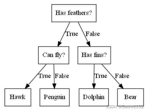
可见，该算法通过树的形式，使用羽毛、飞行、鳍等特征确定某个动物具体的类别。

DecisionTreeClassifier 分类树

直接调用sklearn中的包 DecisionTreeClassifier 进行决策树分类

DecisionTreeClassifier 的简单应用

from sklearn.tree import DecisionTreeClassifier
from sklearn.neighbors import KNeighborsClassifier
from sklearn.datasets import load_breast_cancer
from sklearn.model_selection import train_test_split

#读取乳腺癌数据集
cancer = load_breast_cancer()

#拆分数据集为训练集和测试集
X_train, X_test, y_train, y_test = train_test_split(cancer.data, cancer.target)

#设置DecisionTreeClassifier的最大深度为 4, 防止过拟合的现象产生
tree = DecisionTreeClassifier(max_depth=4, random_state=0)

#训练模型
tree.fit(X_train, y_train)

#输出分类决策树对于不同训练集的预测精度
print('The train: {}'.format(tree.score(X_train,y_train)))
print('The test: {}'.format(tree.score(X_test,y_test)))


1
2
3
4
5
6
7
8
9
10
11
12
13
14
15
16
17
18
19
20
21
22

The train: 0.9882629107981221
The test: 0.951048951048951
1
2

图解决策树分类过程

我们可以分析下该分类决策树，使用export_graphviz函数来可视化分类决策树。

from sklearn.tree import export_graphviz
import graphviz

#绘制图形文件
export_graphviz(tree, out_file='tree.dot', class_names=['malignant', 'benign'], 
                feature_names=cancer.feature_names, impurity=False, filled=True)

with open('tree.dot') as fp:
    dot_grapf = fp.read()
    
graphviz.Source(dot_grapf)

1
2
3
4
5
6
7
8
9
10
11
12

由上图可知，benign类别大多数处于决策树的左侧， malignant类别大多数处于决策树的右侧，由此我们可以得出推论

mean concave points <= 0.051 有效地对数据类别进行了划分，说明该数值能够作为划分类别的重要特征

分类决策树的重要特征

分类决策树的一个很重要的原理就是决策树的特征重要性

对于每个特征来说，均是介于0和1之间的数值，其中 0 表示 ‘根本没有’， 1 表示 ‘能够完全预测目标值’ ，特征值的求和始终为 1。

print('Features:\n{}'.format(cancer.feature_names))
print('Feature importances:\n{}'.format(tree.feature_importances_))
1
2
3

Features:
['mean radius' 'mean texture' 'mean perimeter' 'mean area'
 'mean smoothness' 'mean compactness' 'mean concavity'
 'mean concave points' 'mean symmetry' 'mean fractal dimension'
 'radius error' 'texture error' 'perimeter error' 'area error'
 'smoothness error' 'compactness error' 'concavity error'
 'concave points error' 'symmetry error' 'fractal dimension error'
 'worst radius' 'worst texture' 'worst perimeter' 'worst area'
 'worst smoothness' 'worst compactness' 'worst concavity'
 'worst concave points' 'worst symmetry' 'worst fractal dimension']
Feature importances:
[0.         0.         0.         0.         0.         0.
 0.00780371 0.72350822 0.         0.         0.         0.
 0.         0.0131596  0.         0.         0.         0.
 0.01738099 0.02051472 0.         0.04432579 0.11585585 0.03121485
 0.         0.         0.         0.00542637 0.         0.0208099 ]
1
2
3
4
5
6
7
8
9
10
11
12
13
14
15
16

以上是该决策树的每个特征对应的重要性程度, 可见 mean concave points = 0.72350822，对应的重要性最高

所以决策树的根节点首先以 mean concave points 特征进行分类，然后再根据次级的重要性，依次划分，接下来我们对决策树特征重要性进行可视化

import matplotlib.pyplot as plt
import numpy as np

def plot_feature_importance_cancer(model):
    
    #获取到特征的个数
    n_features = cancer.data.shape[1]
    
    #根据重要性进行绘图
    plt.barh(range(n_features), model.feature_importances_, align='center')
    
    plt.yticks(np.arange(n_features), cancer.feature_names)
    plt.xlabel('Feature importance')
    plt.ylabel('Feature')
    
plot_feature_importance_cancer(tree)

1
2
3
4
5
6
7
8
9
10
11
12
13
14
15
16
17

此处我们可以看到，果然根节点划分是根据最重要的特征 mean concave points 进行划分的，然后越靠近根节点的划分，依据特征的重要性越重要，且特征重要性始终为正数。

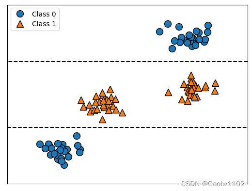
但是我们不能这样表示，如 mean concave points <= 0.051 就是良性(类别0)，否则 mean concave points > 0.051 就是恶性(类别1), 如以下例子

import IPython.display

tree = mglearn.plots.plot_tree_not_monotone()
display(tree)
1
2
3
4

Feature importances: [0. 1.]
1

由以上例子我们便可知，特征重要性仅能代表决策树的切分依据，并不能直接说，‘较小的 mean concave points 对应良性(benign)，较大的 mean concave points 对应恶性(malignant)’

DecisionTreeRegressor 回归树

回归树的用法与分析与分类树十分类似

但是回归树存在一个特殊的特质，即不能外推，也不能在训练集之外进行预测，如下例

DecisionTreeRegressor回归树的简单应用与分析

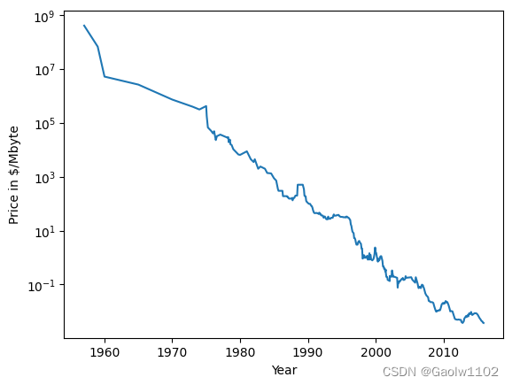
我们利用计算机内存(RAM)历史价格的数据集来研究, X为年号， Y为价格

import pandas as pd

#读取ram价格变化的数据集
ram_prices = pd.read_csv('./dataset/ram_prices.csv')

#绘图，根据价格和日期
plt.semilogy(ram_prices.date, ram_prices.price)
plt.xlabel('Year')
plt.ylabel('Price in $/Mbyte')


1
2
3
4
5
6
7
8
9
10
11

Text(0, 0.5, 'Price in $/Mbyte')
1

我们将利用 2000 年前的历史数据来预测 2000年后的价格，仅以日期作为特征。

通过对比线性回归 LinearRegression和决策树回归 TreeDecisionRegressor，来观测结果

from sklearn.tree import DecisionTreeRegressor
from sklearn.linear_model import LinearRegression

#拆分训练集和测试集
data_train = ram_prices[ram_prices.date < 2000]
data_test = ram_prices[ram_prices.date >= 2000]


#基于日期来预测价格, np.newaxis用来增加维度，对一维数组增加维度
# x[:, np.newaxis] ，放在后面，会给列上增加维度
# x[np.newaxis, :] ，放在前面，会给行上增加维度
X_train = data_train.date[:, np.newaxis]
#我们利用对数变换得到数据和目标之间更简单的关系
y_train = np.log(data_train.price)

#构建模型并训练模型
tree = DecisionTreeRegressor().fit(X_train, y_train)
linear_reg = LinearRegression().fit(X_train, y_train)

#对所有数据进行预测
X_all = ram_prices.date[:, np.newaxis]

pred_tree = tree.predict(X_all)
pred_lr = linear_reg.predict(X_all)

#对数运算逆运算
price_tree = np.exp(pred_tree)
price_lr = np.exp(pred_lr)
1
2
3
4
5
6
7
8
9
10
11
12
13
14
15
16
17
18
19
20
21
22
23
24
25
26
27
28

plt.semilogy(data_train.date, data_train.price, label = 'Training data')              #测试集的日期/价格图
plt.legend()          #绘制曲线标签
1
2

1

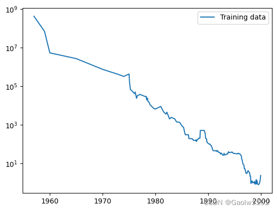
训练集的日期/价格曲线图

plt.semilogy(data_train.date, data_train.price, label = 'Training data')              #测试集的日期/价格图
plt.semilogy(data_test.date, data_test.price, label = 'Test data')                    #测试集的日期/价格图
plt.legend()          #绘制曲线标签
1
2
3

1

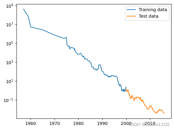
训练集 + 测试集的日期/价格图

plt.semilogy(data_train.date, data_train.price, label = 'Training data')              #测试集的日期/价格图
plt.semilogy(data_test.date, data_test.price, label = 'Test data')                    #测试集的日期/价格图
plt.semilogy(ram_prices.date, price_tree, label = 'Tree prediction')                  #回归决策树的日期/价格图
plt.legend()          #绘制曲线标签
1
2
3
4

1

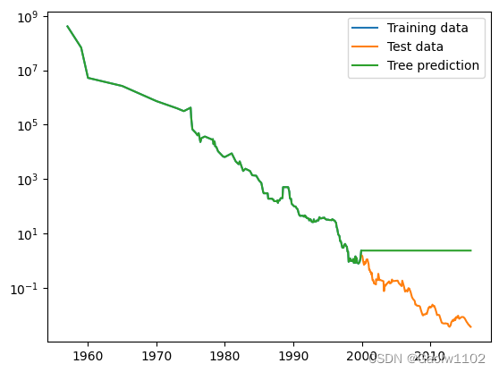
训练集 + 测试集 + 回归树预测的日期/价格图，由此图可见，决策回归树在2000年前完美预测了训练集的价格趋势，而在2000年后，则不能正确预测，即不具备对测试集的外推能力

plt.semilogy(data_train.date, data_train.price, label = 'Training data')              #测试集的日期/价格图
plt.semilogy(data_test.date, data_test.price, label = 'Test data')                    #测试集的日期/价格图
plt.semilogy(ram_prices.date, price_tree, label = 'Tree prediction')                  #回归决策树的日期/价格图
plt.semilogy(ram_prices.date, price_lr, label = 'Linear predction')                  #回归决策树的日期/价格图
plt.legend()          #绘制曲线标签
1
2
3
4
5

1

训练集 + 测试集 + 回归树预测 + 线性回归预测的日期/价格图，此时可见，线性回归模型仍然能够对ram的价格继续进行预测，即可以对训练集外推。

小结

决策树存在两个优点，一是的得到的模型易于可视化、易于理解，二是完全不受数据缩放的影响。

主要缺点在于，可能会出现过拟合现象，即决策树的深度过深，分类过于细化，导致训练集预测完美，测试集预测较差，泛化能力较差。故可用集成方法决策树集成替代决策树。