本文将以周志华《机器学习》中的习题8.3的要求和数据，用python完成一个基于决策树的AdaBoost。

1.题干

从网上下载或自己编程实现AdaBoost，以不剪枝决策树为基学习器，在西瓜数据集3.0α上训练一个AdaBoost集成，并与图8.4进行比较。

西瓜数据集3.0α如下（第一列表示密度，第二列表示含糖量，第三列为数据的标签，表示是否是好瓜）：

0.697,0.460,是
0.774,0.376,是
0.634,0.264,是
0.608,0.318,是
0.556,0.215,是
0.403,0.237,是
0.481,0.149,是
0.437,0.211,是
0.666,0.091,否
0.243,0.267,否
0.245,0.057,否
0.343,0.099,否
0.639,0.161,否
0.657,0.198,否
0.360,0.370,否
0.593,0.042,否
0.719,0.103,否

2.python实现

关于adaboost的理论可以参考这篇博客：Adaboost 算法实例解析
这里直接进行实现。

首先，根据题目要求，要实现一个基于不剪枝决策树的Adaboost学习器，学习器可以对西瓜数据进行二分类。
所以，第一步实现决策树，这里按照信息熵来寻找最优的划分属性。另外，我们还需要注意，因为集成学习过程中有权重的概念，所以实现的决策树也要将权重参与计算。

2.1 决策树实现

首先是获取数据部分，从txt读入数据，具体见代码：

import numpy as np
import matplotlib.pyplot as plt
import matplotlib as mpl
import math
import copy

def get_data():
    x = []
    y = []
    with open("./xigua.txt", 'r') as f:
        for line in f.readlines():
            words = line.split(',')
            instance = []
            for word in words[:2]:
                instance.append(float(word))
            x.append(instance)
            if '是' in words[2]:
                y.append(1)
            elif '否' in words[2]:
                y.append(0)
    return x, y
1
2
3
4
5
6
7
8
9
10
11
12
13
14
15
16
17
18
19
20
21

然后，是基于信息熵的决策树中比较重要的部分，求信息熵。信息熵代表数据集的数据纯度，信息熵越高表示数据的类别越杂，反之越纯。
求信息熵的公式：
（pk表示第k类数据的占比，Y等于类别总数）

def ent(D):
    """
    求信息熵。
    
    Parameters:
    D :  D是一个元组，格式为(w, x, y)。表示数据集，w为权重，x为数据，y为标签。
    
    Returns:
    一个实数，表示信息熵。
    """
    w, x, y = D
    h = 1e-17
    y = np.array(y)
    p0 = np.sum(w * (y == 0)) / np.sum(w)
    p1 = np.sum(w * (y == 1)) / np.sum(w)
    
    return -p0*np.log2(p0 + h) - p1*np.log2(p1 + h)
1
2
3
4
5
6
7
8
9
10
11
12
13
14
15
16
17

接下来是信息增益，简单来说，就是通过一次划分信息熵减少了多少。
信息增益公式如下：
(a表示划分属性，Dv表示将D划分后的第v个数据集，V等于划分后的数据集个数)

另外，我这里的代码没有严格跟公式一样，有个不同的地方：
公式是传入划分属性，然后在函数体内进行划分。这里直接传入的划分好的数据，划分工作交给外部了，反正效果是一样的。

def gain(D, DS):
    """
    求信息增益。
    
    Parameters:
    D :  D是一个元组，格式为(w, x, y)。表示划分前的数据集，w为权重，x为数据，y为标签。
    DS ：DS是一个列表，元素为元组，每个元组格式为(w, x, y)。表示划分后的数据集组成的列表。
    
    Returns:
    一个实数gain，表示信息增益。
    """
    dw, dx, dy = D
    original_size = np.sum(dw)
    
    ent_d = ent(D)
    gain = ent_d
    
    for di in DS:
        w, x, y = di
        gain -= (np.sum(w) / original_size) * ent(di)
        
    return gain
1
2
3
4
5
6
7
8
9
10
11
12
13
14
15
16
17
18
19
20
21
22

接下来就是按照信息增益来找最佳划分属性（best_divider）了，我们需要注意这里的西瓜属性都是离散型数据，所以我们要按照离散型属性的套路来实现。

即对于每个属性，先将训练集按照该属性排序，然后取两两间的中间值看作待选择的divider（比如在本题中就是，对于密度，就将17个西瓜按照密度排序，然后取出16个中间值，同样对于含糖量，将17个西瓜按照含糖量排序，取出16个间隔值，最后能得到32个间隔值，这32个间隔值就是32个divider（divider结构形如 （“密度”， 0.542）））。

然后在得到所有可能的划分依据divider后，按照信息增益来选择增益最大的divider。

def find_best_divider(D, A):
    """
    按照信息增益最大的准则寻找最佳划分。
    
    Parameters:
    D :  同上。
    
    Returns:
    （划分属性，划分属性值）
    """
    w, x, y = D
    best_divider = None
    
    gains = []
    dividers = []
    
    for attr in A: 
        sorted_D = sort_D_by_attr(D, attr)
        sorted_w, sorted_x, sorted_y = sorted_D
        for i in range(len(sorted_x)-1):
            mid_val = (sorted_x[i][attr] + sorted_x[i+1][attr]) / 2.0
            dividers.append((attr, mid_val))
    
    for divider in dividers:
        DS = divide(D, divider)
        gains.append(gain(D, DS))
        
    max_gain = 0
    for i in range(len(gains)):
        if gains[i] > max_gain:
            max_gain = gains[i]
            best_divider = dividers[i]
    
    return best_divider
1
2
3
4
5
6
7
8
9
10
11
12
13
14
15
16
17
18
19
20
21
22
23
24
25
26
27
28
29
30
31
32
33
34

求信息增益前，需要根据每个divider得到划分结果，划分函数如下：

def divide(D, divider):
    """
    按照divider内容对数据集D进行划分。
    
    Parameters:
    D :  同上。
    divider ：（划分属性，划分值）按照划分属性大于和小于划分值情况将D分别划分为D0和D1，并包含进DS
    
    Returns:
    划分完的数据集列表，包含D0和D1
    """
    w, x, y = D
    DS = []
    divider_attr, divider_attr_val = divider
    
    w0, x0, y0 = [],[],[]
    w1, x1, y1 = [],[],[]
    
    for i in range(len(x)):
        if x[i][divider_attr] < divider_attr_val:
            w0.append(w[i])
            x0.append(x[i])
            y0.append(y[i])
        else:
            w1.append(w[i])
            x1.append(x[i])
            y1.append(y[i])
            
    D0 = (w0, x0, y0)
    D1 = (w1, x1, y1)
    DS = [D0, D1]
    return DS
1
2
3
4
5
6
7
8
9
10
11
12
13
14
15
16
17
18
19
20
21
22
23
24
25
26
27
28
29
30
31
32

按照属性进行排序：

def sort_D_by_attr(D, attr):
    sorted_D = copy.deepcopy(D)
    w, x, y = sorted_D
    size = len(x)
    for i in range(size-1):
        for j in range(size-i-1):
            if x[j][attr] > x[j+1][attr]:
                t = x[j]
                x[j] = x[j+1]
                x[j+1] = t
                
                t = w[j]
                w[j] = w[j+1]
                w[j+1] = t
                
                t = y[j]
                y[j] = y[j+1]
                y[j+1] = t
                
    return sorted_D
1
2
3
4
5
6
7
8
9
10
11
12
13
14
15
16
17
18
19
20

然后，是决策树的节点类：

class Node:
    def __init__(self):
        self.attr = None
        self.attr_val = None
        self.less_than_val_child = None
        self.bigger_than_val_child = None
        self.result_category = None
        
    def is_leaf(self):
        if self.attr is None:
            return True
        else:
            return False
        
    def __str__(self):
        return "划分属性：" + str(self.attr) + ' ' + "划分值：" + str(self.attr_val) + ', ' + "结果：" + str(self.result_category)
    
    def show(self):
        if self is None:
            return
        print(self)
        
        if self.less_than_val_child is not None:
            self.less_than_val_child.show()
        if self.bigger_than_val_child is not None:
            self.bigger_than_val_child.show()
    
1
2
3
4
5
6
7
8
9
10
11
12
13
14
15
16
17
18
19
20
21
22
23
24
25
26
27

然后，就可以实现决策树的训练过程了，整个过程是一个递归过程，递归返回的情况有三种，一种是当前数据集类别相同，则不用划分。第二种是当前数据集的所有属性都相同，没法划分，第三种是当前的数据集是空的，那么不能划分。

def tree_generate(D, A):
    '''
    Parameters:
    D为数据集，A为属性集
    '''
    w, x, y = D
    
    node = Node()
    if is_same_y(D):
        node.result_category = y[0]
        return node
    if A is None or len(A) == 0 or is_same_val_in_A(D, A):
        most_possible_y = get_most_possible_y(D)
        node.result_category = most_possible_y
        return node
    
    attr, attr_val = find_best_divider(D, A)
    
    divider = (attr, attr_val)
    DS = divide(D, divider)
    node.attr = attr
    node.attr_val = attr_val
    new_A = A
#     new_A.remove(attr)
    
    if DS[0] is None:
        node0 = Node()
        node0.result_category = get_most_possible_y(D)
        node.less_than_val_child = node0
    else:
        node.less_than_val_child = tree_generate(DS[0], new_A)
        
    if DS[1] is None:
        node1 = Node()
        node1.result_category = get_most_possible_y(D)
        node.bigger_than_val_child = node1
    else:
        node.bigger_than_val_child = tree_generate(DS[1], new_A)
    
    return node
1
2
3
4
5
6
7
8
9
10
11
12
13
14
15
16
17
18
19
20
21
22
23
24
25
26
27
28
29
30
31
32
33
34
35
36
37
38
39
40

其他函数：

def get_most_possible_y(D):
    w, x, y = D
    y = np.array(y)
    
    cnt_0 = np.sum(w * (y == 0))
    cnt_1 = np.sum(w * (y == 1))
    
    if cnt_0 > cnt_1:
        return 0
    else:
        return 1

def is_same_val_in_A(D, A):
    w, x, y = D
    for a in A:
        first_val = x[0][a]
        for xi in x:
            if xi[a] != first_val:
                return False
    
    return True

def is_same_y(D):
    w, x, y = D
    for yi in y:
        if yi != y[0]:
            return False
    return True
1
2
3
4
5
6
7
8
9
10
11
12
13
14
15
16
17
18
19
20
21
22
23
24
25
26
27
28

决策树训练函数：

def train_1(D):
    w, x, y = D
    n = len(x[0])
    A = list(range(n))
    node = tree_generate(D, A)
#     node = tree_stool_generate(D, A)
    return node
1
2
3
4
5
6
7

至此，决策树的代码就写完了，可以通过以下代码简单测试一下：

x, y = get_data()
w = [1/17 for _ in range(17)]
A = list(range(2))
D = (w, x, y)
node = tree_generate(D, A)

node.show()
1
2
3
4
5
6
7

就是对训练数据进行一次划分（权重均分），可以看到，生成的决策树和《机器学习》P90 图4.3 中的结果一致：
（这里没有对树进行画图展示，直接按照先序遍历循序打印了节点）

2.2 AdaBoost实现

参数T表示集成学习包含几个基学习器，也就是几个决策树。首先获取数据，然后进入for循环，循环T次，每一次将训练数据，训练标签，权重包含进D中，然后进行训练，得到学习器ht，然后计算一下ht的错误率et。这里主要要避免et=0的情况，防止一会除0。如果et>0.5则停止训练。然后将学习器ht存入学习器列表h_list，然后计算该学习器的权重alpha[t]，表示该学习器最终的"话语权"。

然后就是adaboost的重点，更新权重，adaboost通过 “降低预测正确样本的权重，提高预测错误样本的权重” 来保证这些基学习器的多样性，更新权重的公式如下：
Dt(x)表示数据x在第t轮训练的权重（对应代码中的变量w，w[i]表示第i条数据的权重，注意没有下标t，因为每次训练直接覆盖上次的权重了）。
Zt就是一个规范化因子，用于保证权重加和等于1（对应代码中的变量Z）。

def adaboost_1_train(T):
    alpha = []
    h_list = []
    
    x, y = get_data()
    N = len(y)
    w = [1/N for _ in range(N)]
    for t in range(T):
        print('w[', t, '] : \n', w, '\n')
        D = (w, x, y)
        ht = train_1(D)
        et = loss(ht, D)
        if et == 0:
            et = 0.00001
        if et > 0.5:
            break
        h_list.append(ht)
        alpha.append(0.5 * math.log((1-et)/et))
        
        Z = 0
        for i in range(N):
            predict_y = predict(ht, x[i])
            if predict_y == y[i]:
                Z += w[i] * math.exp(-alpha[t])
            else:
                Z += w[i] * math.exp(alpha[t])
            
        for i in range(N):
            w[i] = w[i] / Z
            predict_y = predict(ht, x[i])
            if predict_y == y[i]:
                w[i] *=  math.exp(-alpha[t])
            else:
                w[i] *=  math.exp(alpha[t])
        
    return h_list, alpha    
1
2
3
4
5
6
7
8
9
10
11
12
13
14
15
16
17
18
19
20
21
22
23
24
25
26
27
28
29
30
31
32
33
34
35
36

计算错误率：

def loss(h, D):
    w, x, y = D
    loss = 0
    for i in range(len(x)):
        predict_y = predict(h, x[i])
        if predict_y != y[i]:
            loss += w[i]
    
    return loss
1
2
3
4
5
6
7
8
9

集成学习器预测：

def adaboost_predict(model, x):
    h_list, alpha = model
    p_pos = 0
    p_neg = 0
    for i in range(len(h_list)):
        predict_y = predict(h_list[i], x)
        p_pos += predict_y * alpha[i]
        p_neg += (1-predict_y) * alpha[i]
        
    return p_pos > p_neg
1
2
3
4
5
6
7
8
9
10

决策树的分类边界的可视化：

def model_plot(h):
    x, y = get_data()
    train_label = y
    train_value = x
    x1 = [mapi[0] for mapi in train_value]
    x2 = [mapi[1] for mapi in train_value]
    x = np.c_[x1,x2]

    np_x = np.asarray(x)
    np_y = np.asarray(train_label)
    N, M = 100, 100

    x1_min, x2_min = np_x.min(axis=0)
    x1_max, x2_max = np_x.max(axis=0)

    x1_min -= 0.1
    x2_min -= 0.1
    x1_max += 0.1 
    x2_max += 0.1

    t1 = np.linspace(x1_min, x1_max, N)
    t2 = np.linspace(x2_min, x2_max, M)

    grid_x, grid_y = np.meshgrid(t1,t2)

    grid = np.stack([grid_x.flat, grid_y.flat], axis=1)
    y_fake = np.zeros((N*M,))

    y_predict = []
    for xi in grid:
        y_predict.append(predict(h, xi))

    cm_light = mpl.colors.ListedColormap(['#A0FFA0', '#FFA0A0'])
    plt.pcolormesh(grid_x, grid_y, np.array(y_predict).reshape(grid_x.shape), cmap=cm_light)
    plt.scatter(x[:,0], x[:,1], s=30, c=train_label, marker='o')

    plt.show()
1
2
3
4
5
6
7
8
9
10
11
12
13
14
15
16
17
18
19
20
21
22
23
24
25
26
27
28
29
30
31
32
33
34
35
36
37

3. 结果

至此，已经完成了adaboost的全部实现，可以开始测试。
令基学习器的数量为11，进行训练，然后分别打印权重的变化过程，并绘制11个决策树的分类边界。

# 主程序
# （不剪枝决策树, 集成训练， 分开展示）
model = adaboost_1_train(11)
h_list, alpha = model

for h in h_list:
    model_plot(h)
1
2
3
4
5
6
7

观察结果：

w[ 0 ] :
[0.058823529411764705, 0.058823529411764705, 0.058823529411764705, 0.058823529411764705, 0.058823529411764705, 0.058823529411764705, 0.058823529411764705, 0.058823529411764705, 0.058823529411764705, 0.058823529411764705, 0.058823529411764705, 0.058823529411764705, 0.058823529411764705, 0.058823529411764705, 0.058823529411764705, 0.058823529411764705, 0.058823529411764705]
w[ 1 ] :
[0.058823529411764684, 0.058823529411764684, 0.058823529411764684, 0.058823529411764684, 0.058823529411764684, 0.058823529411764684, 0.058823529411764684, 0.058823529411764684, 0.058823529411764684, 0.058823529411764684, 0.058823529411764684, 0.058823529411764684, 0.058823529411764684, 0.058823529411764684, 0.058823529411764684, 0.058823529411764684, 0.058823529411764684]
w[ 2 ] :
[0.0588235294117647, 0.0588235294117647, 0.0588235294117647, 0.0588235294117647, 0.0588235294117647, 0.0588235294117647, 0.0588235294117647, 0.0588235294117647, 0.0588235294117647, 0.0588235294117647, 0.0588235294117647, 0.0588235294117647, 0.0588235294117647, 0.0588235294117647, 0.0588235294117647, 0.0588235294117647, 0.0588235294117647]
w[ 3 ] :
[0.058823529411764684, 0.058823529411764684, 0.058823529411764684, 0.058823529411764684, 0.058823529411764684, 0.058823529411764684, 0.058823529411764684, 0.058823529411764684, 0.058823529411764684, 0.058823529411764684, 0.058823529411764684, 0.058823529411764684, 0.058823529411764684, 0.058823529411764684, 0.058823529411764684, 0.058823529411764684, 0.058823529411764684]
w[ 4 ] :
[0.0588235294117647, 0.0588235294117647, 0.0588235294117647, 0.0588235294117647, 0.0588235294117647, 0.0588235294117647, 0.0588235294117647, 0.0588235294117647, 0.0588235294117647, 0.0588235294117647, 0.0588235294117647, 0.0588235294117647, 0.0588235294117647, 0.0588235294117647, 0.0588235294117647, 0.0588235294117647, 0.0588235294117647]
w[ 5 ] :
[0.058823529411764684, 0.058823529411764684, 0.058823529411764684, 0.058823529411764684, 0.058823529411764684, 0.058823529411764684, 0.058823529411764684, 0.058823529411764684, 0.058823529411764684, 0.058823529411764684, 0.058823529411764684, 0.058823529411764684, 0.058823529411764684, 0.058823529411764684, 0.058823529411764684, 0.058823529411764684, 0.058823529411764684]

w[ 6 ] : [0.0588235294117647, 0.0588235294117647,
0.0588235294117647, 0.0588235294117647, 0.0588235294117647, 0.0588235294117647, 0.0588235294117647, 0.0588235294117647, 0.0588235294117647, 0.0588235294117647, 0.0588235294117647, 0.0588235294117647, 0.0588235294117647, 0.0588235294117647, 0.0588235294117647, 0.0588235294117647, 0.0588235294117647]

w[ 7 ] : [0.058823529411764684, 0.058823529411764684,
0.058823529411764684, 0.058823529411764684, 0.058823529411764684, 0.058823529411764684, 0.058823529411764684, 0.058823529411764684, 0.058823529411764684, 0.058823529411764684, 0.058823529411764684, 0.058823529411764684, 0.058823529411764684, 0.058823529411764684, 0.058823529411764684, 0.058823529411764684, 0.058823529411764684]

w[ 8 ] : [0.0588235294117647, 0.0588235294117647,
0.0588235294117647, 0.0588235294117647, 0.0588235294117647, 0.0588235294117647, 0.0588235294117647, 0.0588235294117647, 0.0588235294117647, 0.0588235294117647, 0.0588235294117647, 0.0588235294117647, 0.0588235294117647, 0.0588235294117647, 0.0588235294117647, 0.0588235294117647, 0.0588235294117647]

w[ 9 ] : [0.058823529411764684, 0.058823529411764684,
0.058823529411764684, 0.058823529411764684, 0.058823529411764684, 0.058823529411764684, 0.058823529411764684, 0.058823529411764684, 0.058823529411764684, 0.058823529411764684, 0.058823529411764684, 0.058823529411764684, 0.058823529411764684, 0.058823529411764684, 0.058823529411764684, 0.058823529411764684, 0.058823529411764684]

w[ 10 ] : [0.0588235294117647, 0.0588235294117647,
0.0588235294117647, 0.0588235294117647, 0.0588235294117647, 0.0588235294117647, 0.0588235294117647, 0.0588235294117647, 0.0588235294117647, 0.0588235294117647, 0.0588235294117647, 0.0588235294117647, 0.0588235294117647, 0.0588235294117647, 0.0588235294117647, 0.0588235294117647, 0.0588235294117647]

分类边界图像：
第一个：

（另外10个图像都一样）

可以看到，每轮训练的权重没有任何变化，并且训练出的决策树都是相同的。这种现象发生的原因就是，第一个基学习器训练后，其准确率已经达到100%，也就是说没有预测错误的样本，那么权重也就不会发生改变，进而后面10个基学习器的训练结果就和第一个一样了。这也验证了集成学习的特点，集成学习可以将多个弱学习器集成变成一个强学习器，但是如果基学习器就是强学习器（或者说在当前数据集上表现足够好），那么集成学习的效果就不显著了。

4.附加

为了展示出adaboost效果，这里将基学习器改成弱学习器，把不剪枝决策树改为决策树桩（只进行一次划分的决策树），重新实验。

决策树桩的实现：

def tree_stool_generate(D, A):
    node = Node()
    attr, attr_val = find_best_divider(D, A)
    node.attr = attr
    node.attr_val = attr_val
    
    DS = divide(D, (attr, attr_val))
    
    child_l = Node()
    child_l.result_category = get_most_possible_y(DS[0])
    child_b = Node()
    child_b.result_category = get_most_possible_y(DS[1])
    
    node.less_than_val_child = child_l
    node.bigger_than_val_child = child_b
    
    return node
1
2
3
4
5
6
7
8
9
10
11
12
13
14
15
16
17

决策树桩训练：

def train_2(D):
    w, x, y = D
    n = len(x[0])
    A = list(range(n))
#     node = tree_generate(D, A)
    node = tree_stool_generate(D, A)
    return node
1
2
3
4
5
6
7

决策树桩版的adaboost：

def adaboost_2_train(T):
    alpha = []
    h_list = []
    
    x, y = get_data()
    N = len(y)
    w = [1/N for _ in range(N)]
    for t in range(T):
        print('w[', t, '] : \n', w, '\n')
        D = (w, x, y)
        ht = train_2(D)
        et = loss(ht, D)
        if et == 0:
            et = 0.00001
        if et > 0.5:
            break
        h_list.append(ht)
        alpha.append(0.5 * math.log((1-et)/et))
        
        Z = 0
        for i in range(N):
            predict_y = predict(ht, x[i])
            if predict_y == y[i]:
                Z += w[i] * math.exp(-alpha[t])
            else:
                Z += w[i] * math.exp(alpha[t])
            
        for i in range(N):
            w[i] = w[i] / Z
            predict_y = predict(ht, x[i])
            if predict_y == y[i]:
                w[i] *=  math.exp(-alpha[t])
            else:
                w[i] *=  math.exp(alpha[t])
        
    return h_list, alpha    
1
2
3
4
5
6
7
8
9
10
11
12
13
14
15
16
17
18
19
20
21
22
23
24
25
26
27
28
29
30
31
32
33
34
35
36

然后，编写测试程序，进行测试和展示（同样是11个基学习器）：

# 主程序
# （决策树桩, 集成训练， 分开展示）

model = adaboost_2_train(11)
h_list, alpha = model

for h in h_list:
    model_plot(h)
    
x, y = get_data()
x = np.array(x)
y = np.array(y)

for i in range(len(y)):
    plt.scatter(x[:, 0], x[:, 1], c=y, marker='o')
for h in h_list:
    if h.attr == 0:
        p_a = [h.attr_val, 0.01]
        p_b = [h.attr_val, 0.6]
    else:
        p_a = [0.1, h.attr_val]
        p_b = [0.8, h.attr_val]
    plt.plot([p_a[0], p_b[0]], [p_a[1], p_b[1]], 'g-')
plt.show()
1
2
3
4
5
6
7
8
9
10
11
12
13
14
15
16
17
18
19
20
21
22
23
24

运行结果：
权重变化过程：

w[ 0 ] :
[0.058823529411764705, 0.058823529411764705, 0.058823529411764705, 0.058823529411764705, 0.058823529411764705, 0.058823529411764705, 0.058823529411764705, 0.058823529411764705, 0.058823529411764705, 0.058823529411764705, 0.058823529411764705, 0.058823529411764705, 0.058823529411764705, 0.058823529411764705, 0.058823529411764705, 0.058823529411764705, 0.058823529411764705]

w[ 1 ] : [0.03846153846153847, 0.03846153846153847,
0.03846153846153847, 0.03846153846153847, 0.03846153846153847, 0.03846153846153847, 0.03846153846153847, 0.03846153846153847, 0.03846153846153847, 0.12500000000000003, 0.03846153846153847, 0.03846153846153847, 0.12500000000000003, 0.12500000000000003, 0.12500000000000003, 0.03846153846153847, 0.03846153846153847]

w[ 2 ] : [0.062499999999999986, 0.062499999999999986,
0.062499999999999986, 0.062499999999999986, 0.062499999999999986, 0.062499999999999986, 0.062499999999999986, 0.062499999999999986, 0.02777777777777778, 0.09027777777777778, 0.02777777777777778, 0.02777777777777778, 0.09027777777777778, 0.09027777777777778, 0.09027777777777778, 0.02777777777777778, 0.02777777777777778]

w[ 3 ] : [0.042452830188679236, 0.042452830188679236,
0.042452830188679236, 0.042452830188679236, 0.042452830188679236, 0.042452830188679236, 0.042452830188679236, 0.042452830188679236, 0.05263157894736844, 0.06132075471698114, 0.01886792452830189, 0.01886792452830189, 0.1710526315789474, 0.1710526315789474, 0.06132075471698114, 0.05263157894736844, 0.05263157894736844]

w[ 4 ] : [0.025423728813559313, 0.025423728813559313,
0.025423728813559313, 0.025423728813559313, 0.025423728813559313, 0.025423728813559313, 0.1285714285714285, 0.025423728813559313, 0.031519476657746064, 0.1857142857142857, 0.011299435028248588, 0.011299435028248588, 0.1024382991376747, 0.1024382991376747, 0.1857142857142857, 0.031519476657746064, 0.031519476657746064]

w[ 5 ] : [0.018145161290322575, 0.018145161290322575,
0.018145161290322575, 0.018145161290322575, 0.018145161290322575, 0.018145161290322575, 0.09176267281105986, 0.018145161290322575, 0.052631578947368425, 0.13254608294930875, 0.008064516129032258, 0.008064516129032258, 0.17105263157894737, 0.17105263157894737, 0.13254608294930875, 0.052631578947368425, 0.052631578947368425]

w[ 6 ] : [0.04146919431279622, 0.04146919431279622,
0.04146919431279622, 0.04146919431279622, 0.04146919431279622, 0.04146919431279622, 0.20971563981042654, 0.04146919431279622, 0.0336854523863116, 0.0848326205574399, 0.005161480607580002, 0.005161480607580002, 0.1094777202555127, 0.1094777202555127, 0.0848326205574399, 0.0336854523863116, 0.0336854523863116]

w[ 7 ] : [0.030492583673288998, 0.030492583673288998,
0.030492583673288998, 0.030492583673288998, 0.030492583673288998, 0.030492583673288998, 0.15420535171920433, 0.030492583673288998, 0.05263157894736842, 0.06237800910865321, 0.003795272175233137, 0.003795272175233137, 0.17105263157894735, 0.17105263157894735, 0.06237800910865321, 0.05263157894736842, 0.05263157894736842]

w[ 8 ] : [0.0619860413620309, 0.0619860413620309,
0.02021956227836733, 0.02021956227836733, 0.02021956227836733, 0.02021956227836733, 0.10225321495060045, 0.02021956227836733, 0.03489987925383093, 0.12680348422154747, 0.007715118553244956, 0.007715118553244956, 0.11342460757495053, 0.11342460757495053, 0.12680348422154747, 0.10699071172635338, 0.03489987925383093]

w[ 9 ] : [0.03890423725611639, 0.03890423725611639,
0.0497159090909091, 0.0497159090909091, 0.0497159090909091, 0.0497159090909091, 0.25142045454545453, 0.0497159090909091, 0.021904176373691363, 0.07958554420736225, 0.0048422321551632825, 0.0048422321551632825, 0.07118857321449694, 0.07118857321449694, 0.07958554420736225, 0.06715047358633955, 0.021904176373691363]

w[ 10 ] : [0.026052036683798175, 0.026052036683798175,
0.033292021094723095, 0.033292021094723095, 0.033292021094723095, 0.033292021094723095, 0.16836250667902816, 0.033292021094723095, 0.043231476633221015, 0.053294079602197446, 0.0032425776376825907, 0.0032425776376825907, 0.1405022990579683, 0.1405022990579683, 0.053294079602197446, 0.1325324486176212, 0.043231476633221015]

11个决策树桩的分类边界（最后一个图是11个边界放在一张图中）：

可以看到，使用决策树桩后，基学习器的训练结果发生了变化，同时权重也发生了变化。

（其中出现了全是绿色的结果，这种结果表明决策树按照某个值划分数据集，然后形成左右节点后，认为左右节点都是正例。这种情况就像是，密度>0.5的是好瓜，密度<0.5的也是好瓜。其原因就是，我在判断叶子节点的类别结果使用的算法是，看哪个类的带权占比大，而如果正例的权重都比较大，而反例都比较小的时候，就会发生这个现象）

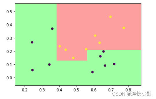
然后，对集成学习器进行集成测试：

# 主程序
# （决策树桩, 集成展示）

x, y = get_data()
train_label = y
train_value = x
x1 = [mapi[0] for mapi in train_value]
x2 = [mapi[1] for mapi in train_value]
x = np.c_[x1,x2]

np_x = np.asarray(x)
np_y = np.asarray(train_label)
N, M = 100, 100

x1_min, x2_min = np_x.min(axis=0)
x1_max, x2_max = np_x.max(axis=0)

x1_min -= 0.1
x2_min -= 0.1
x1_max += 0.1 
x2_max += 0.1

t1 = np.linspace(x1_min, x1_max, N)
t2 = np.linspace(x2_min, x2_max, M)

grid_x, grid_y = np.meshgrid(t1,t2)

grid = np.stack([grid_x.flat, grid_y.flat], axis=1)
y_fake = np.zeros((N*M,))

y_predict = []
for xi in grid:
    y_predict.append(adaboost_predict(model, xi))

cm_light = mpl.colors.ListedColormap(['#A0FFA0', '#FFA0A0'])
plt.pcolormesh(grid_x, grid_y, np.array(y_predict).reshape(grid_x.shape), cmap=cm_light)
plt.scatter(x[:,0], x[:,1], s=30, c=train_label, marker='o')

plt.show()
1
2
3
4
5
6
7
8
9
10
11
12
13
14
15
16
17
18
19
20
21
22
23
24
25
26
27
28
29
30
31
32
33
34
35
36
37
38
39

运行结果：

可以看到，对训练数据的预测准确率100%，与书中图8.4结果相同。