推荐系统之简单线性回归

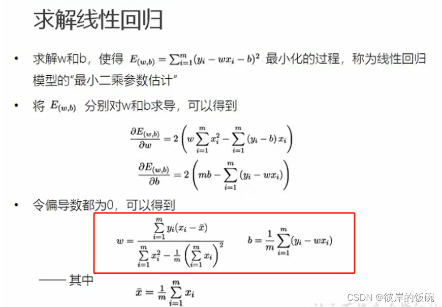
1.简单线性回归（最小二乘法）

import numpy as np
import matplotlib.pyplot as plt

#引入数据
point=np.genfromtxt('data.csv',delimiter=',')
#point[0,0]
x=point[:,0]
y=point[:,1]

plt.scatter(x,y)
plt.show()
1
2
3
4
5
6
7
8
9
10
11

#定义损失函数
def cost_function(w,b,point):
    length=len(point)
    cost_value=0
    for i in range(length):
        zhen=point[i,1]
        jia=point[i,0]*w+b
        cost_value+=(zhen-jia)**2
    return cost_value/length

#求平均值的函数
def average(point):
    length=len(point)
    value=0
    for i in range(length):
        value+=point[i]
    return value/length
1
2
3
4
5
6
7
8
9
10
11
12
13
14
15
16
17

#根据公式求出所谓的w，b   拟合函数
def fit(point):
    average_x=average(point[:,0])
    length=len(point)
    w=0
    b=0
    totalx2=0
    totalx=0
    totalshang=0
    totalb=0
    for i in range(length):
        totalx2+=point[i,0]**2
        totalx+=point[i,0]
        totalshang+=point[i,1]*(point[i,0]-average_x)
    w=totalshang/(totalx2-(totalx**2)/length)
    for i in range(length):
        totalb+=point[i,1]-w*point[i,0]
    b=totalb/length
    return w,b
1
2
3
4
5
6
7
8
9
10
11
12
13
14
15
16
17
18
19

#测试
w,b=fit(point)
print("w的值是:",w)
print("b的值是：",b)
cost=cost_function(w,b,point)
print("他的损失函数值为:",cost)

'''
w的值是: 1.3224310227553846
b的值是： 7.991020982269173
他的损失函数值为: 110.25738346621313
'''

#画出拟合曲线
plt.scatter(x,y)
pred_y=w*x+b
plt.plot(x,pred_y,c="r")
plt.show()
1
2
3
4
5
6
7
8
9
10
11
12
13
14
15
16
17
18

2.梯度下降书写

损失函数，与导入数据方式与上面相同

• 定义模型的超参数

#定义模型的超参数
alpha=0.0001
initial_w=0
initial_b=0
num_list=100    
#迭代100次
1
2
3
4
5
6

以手工和运用EViews软件(或其他软件)：简单线性回归

application/msword 0星 超过10%的资源 350KB

下载

• 定义梯度下降算法以及每一步下降的细节

#定义梯度下降算法
def grad_decs(point,initial_b,initial_w,alpha,num_list):
    w=initial_w
    b=initial_b
    cost_list=[]
    for i in range(num_list):
        cost_list.append(cost_function(w,b,point))
        w,b=step_grad_decs(w,b,alpha,point)
    
    return [w,b,cost_list]

#定义每一步下降的细节函数
def step_grad_decs(w,b,alpha,point):
    current_w=w
    current_b=b
    M=len(point)
    total_w=0
    total_b=0
    for i in range(M):
        total_w+=(w*point[i,0]+b-point[i,1])*point[i,0]
        total_b+=w*point[i,0]+b-point[i,1]
    w=w-alpha*(2/M*total_w)
    b=b-alpha*(2/M*total_b)
    return w,b
1
2
3
4
5
6
7
8
9
10
11
12
13
14
15
16
17
18
19
20
21
22
23
24

• 测试，运行梯度下降算法计算最优w与b

#测试：运行梯度下降算法计算最优w与b
w,b,cost_list=grad_decs( point,initial_b,initial_w,alpha,num_list )
print("w is: ", w)
print("b is: ", b)

cost = cost_function(w, b, point)

print("cost is: ", cost)

plt.plot(cost_list)
plt.show()
1
2
3
4
5
6
7
8
9
10
11

• 画出拟合曲线

#画出拟合曲线

plt.scatter(x,y)
pred_y=w*x+b

plt.plot(x,pred_y,c="r")
plt.show()
1
2
3
4
5
6
7

3. 使用sklearn库来实现线性回归

• 调库，创建初始模型

from sklearn.linear_model import LinearRegression
lr=LinearRegression()

x_new=x.reshape(-1,1)
y_new=y.reshape(-1,1)

lr.fit(x_new,y_new)
1
2
3
4
5
6
7

• 从训练好的模型中提取系数与截距

w=lr.coef_
b=lr.intercept_
print("w is: ", w)
print("b is: ", b)

cost = cost_function(w, b, point)

print("cost is: ", cost)
1
2
3
4
5
6
7
8