-
Python数据分析与机器学习30-SVM实例
一. 通过sklearn提供的make_blobs方法来画图
1.1 简单的画图
代码:
import numpy as np import matplotlib.pyplot as plt from scipy import stats import seaborn as sns; #随机来点数据 from sklearn.datasets._samples_generator import make_blobs sns.set() # 通过sklearn提供的make_blobs方法来画图 X, y = make_blobs(n_samples=50, centers=2,random_state=0, cluster_std=0.60) plt.scatter(X[:, 0], X[:, 1], c=y, s=50, cmap='autumn') plt.show()- 1
- 2
- 3
- 4
- 5
- 6
- 7
- 8
- 9
- 10
- 11
- 12
- 13
- 14
测试记录:

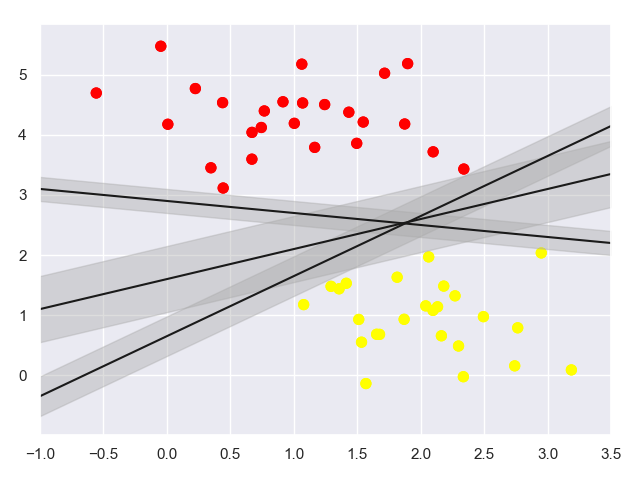
1.2 随便的画几条分割线
代码:
import numpy as np import matplotlib.pyplot as plt from scipy import stats import seaborn as sns; #随机来点数据 from sklearn.datasets._samples_generator import make_blobs sns.set() # 通过sklearn提供的make_blobs方法来画图 X, y = make_blobs(n_samples=50, centers=2,random_state=0, cluster_std=0.60) plt.scatter(X[:, 0], X[:, 1], c=y, s=50, cmap='autumn') # 随便的画几条分割线 xfit = np.linspace(-1, 3.5) plt.scatter(X[:, 0], X[:, 1], c=y, s=50, cmap='autumn') plt.plot([0.6], [2.1], 'x', color='red', markeredgewidth=2, markersize=10) for m, b in [(1, 0.65), (0.5, 1.6), (-0.2, 2.9)]: plt.plot(xfit, m * xfit + b, '-k') plt.xlim(-1, 3.5); plt.show()- 1
- 2
- 3
- 4
- 5
- 6
- 7
- 8
- 9
- 10
- 11
- 12
- 13
- 14
- 15
- 16
- 17
- 18
- 19
- 20
- 21
- 22
- 23
- 24
测试记录:

1.3 SVM最小化 雷区
代码:
import numpy as np import matplotlib.pyplot as plt from scipy import stats import seaborn as sns; #随机来点数据 from sklearn.datasets._samples_generator import make_blobs sns.set() # 通过sklearn提供的make_blobs方法来画图 X, y = make_blobs(n_samples=50, centers=2,random_state=0, cluster_std=0.60) plt.scatter(X[:, 0], X[:, 1], c=y, s=50, cmap='autumn') # 使用SVM来 最小化雷区 xfit = np.linspace(-1, 3.5) plt.scatter(X[:, 0], X[:, 1], c=y, s=50, cmap='autumn') for m, b, d in [(1, 0.65, 0.33), (0.5, 1.6, 0.55), (-0.2, 2.9, 0.2)]: yfit = m * xfit + b plt.plot(xfit, yfit, '-k') plt.fill_between(xfit, yfit - d, yfit + d, edgecolor='none', color='#AAAAAA', alpha=0.4) plt.xlim(-1, 3.5); plt.show()- 1
- 2
- 3
- 4
- 5
- 6
- 7
- 8
- 9
- 10
- 11
- 12
- 13
- 14
- 15
- 16
- 17
- 18
- 19
- 20
- 21
- 22
- 23
- 24
- 25
- 26
测试记录:
二. 训练一个基本的SVM
2.1 训练一个基本的SVM
代码:
import numpy as np import matplotlib.pyplot as plt from scipy import stats import seaborn as sns; #随机来点数据 from sklearn.datasets._samples_generator import make_blobs # 支持向量机 from sklearn.svm import SVC sns.set() # 通过sklearn提供的make_blobs方法来画图 X, y = make_blobs(n_samples=50, centers=2,random_state=0, cluster_std=0.60) # 训练一个基本的SVM model = SVC(kernel='linear') model.fit(X, y) # 绘图函数 def plot_svc_decision_function(model, ax=None, plot_support=True): """Plot the decision function for a 2D SVC""" if ax is None: ax = plt.gca() xlim = ax.get_xlim() ylim = ax.get_ylim() # create grid to evaluate model x = np.linspace(xlim[0], xlim[1], 30) y = np.linspace(ylim[0], ylim[1], 30) Y, X = np.meshgrid(y, x) xy = np.vstack([X.ravel(), Y.ravel()]).T P = model.decision_function(xy).reshape(X.shape) # plot decision boundary and margins ax.contour(X, Y, P, colors='k', levels=[-1, 0, 1], alpha=0.5, linestyles=['--', '-', '--']) # plot support vectors if plot_support: ax.scatter(model.support_vectors_[:, 0], model.support_vectors_[:, 1], s=300, linewidth=1, facecolors='none'); ax.set_xlim(xlim) ax.set_ylim(ylim) plt.scatter(X[:, 0], X[:, 1], c=y, s=50, cmap='autumn') plot_svc_decision_function(model); plt.show()- 1
- 2
- 3
- 4
- 5
- 6
- 7
- 8
- 9
- 10
- 11
- 12
- 13
- 14
- 15
- 16
- 17
- 18
- 19
- 20
- 21
- 22
- 23
- 24
- 25
- 26
- 27
- 28
- 29
- 30
- 31
- 32
- 33
- 34
- 35
- 36
- 37
- 38
- 39
- 40
- 41
- 42
- 43
- 44
- 45
- 46
- 47
- 48
- 49
- 50
测试记录:

这条线就是我们希望得到的决策边界啦
观察发现有3个点做了特殊的标记,它们恰好都是边界上的点
它们就是我们的support vectors(支持向量)
在Scikit-Learn中, 它们存储在这个位置 support_vectors_(一个属性)
2.2 观察数据点变化对SVM的影响
接下来我们尝试一下,用不同多的数据点,看看效果会不会发生变化
分别使用60个和120个数据点
代码:
import numpy as np import matplotlib.pyplot as plt from scipy import stats import seaborn as sns; #随机来点数据 from sklearn.datasets._samples_generator import make_blobs # 支持向量机 from sklearn.svm import SVC sns.set() # 绘图函数 def plot_svc_decision_function(model, ax=None, plot_support=True): """Plot the decision function for a 2D SVC""" if ax is None: ax = plt.gca() xlim = ax.get_xlim() ylim = ax.get_ylim() # create grid to evaluate model x = np.linspace(xlim[0], xlim[1], 30) y = np.linspace(ylim[0], ylim[1], 30) Y, X = np.meshgrid(y, x) xy = np.vstack([X.ravel(), Y.ravel()]).T P = model.decision_function(xy).reshape(X.shape) # plot decision boundary and margins ax.contour(X, Y, P, colors='k', levels=[-1, 0, 1], alpha=0.5, linestyles=['--', '-', '--']) # plot support vectors if plot_support: ax.scatter(model.support_vectors_[:, 0], model.support_vectors_[:, 1], s=300, linewidth=1, facecolors='none'); ax.set_xlim(xlim) ax.set_ylim(ylim) def plot_svm(N=10, ax=None): X, y = make_blobs(n_samples=200, centers=2, random_state=0, cluster_std=0.60) X = X[:N] y = y[:N] model = SVC(kernel='linear', C=1E10) model.fit(X, y) ax = ax or plt.gca() ax.scatter(X[:, 0], X[:, 1], c=y, s=50, cmap='autumn') ax.set_xlim(-1, 4) ax.set_ylim(-1, 6) plot_svc_decision_function(model, ax) fig, ax = plt.subplots(1, 2, figsize=(16, 6)) fig.subplots_adjust(left=0.0625, right=0.95, wspace=0.1) for axi, N in zip(ax, [60, 120]): plot_svm(N, axi) axi.set_title('N = {0}'.format(N)) plt.show()- 1
- 2
- 3
- 4
- 5
- 6
- 7
- 8
- 9
- 10
- 11
- 12
- 13
- 14
- 15
- 16
- 17
- 18
- 19
- 20
- 21
- 22
- 23
- 24
- 25
- 26
- 27
- 28
- 29
- 30
- 31
- 32
- 33
- 34
- 35
- 36
- 37
- 38
- 39
- 40
- 41
- 42
- 43
- 44
- 45
- 46
- 47
- 48
- 49
- 50
- 51
- 52
- 53
- 54
- 55
- 56
- 57
- 58
- 59
- 60
- 61
测试记录:

左边是60个点的结果,右边的是120个点的结果
观察发现,只要支持向量没变,其他的数据怎么加无所谓!三. 引入核函数的SVM
首先我们先用线性的核来看一下在下面这样比较难的数据集上还能分了吗?
3.1 线性不可分的例子
代码:
import numpy as np import matplotlib.pyplot as plt from scipy import stats import seaborn as sns; #随机来点数据 from sklearn.datasets._samples_generator import make_blobs # 支持向量机 from sklearn.svm import SVC from sklearn.datasets._samples_generator import make_circles sns.set() # 绘图函数 def plot_svc_decision_function(model, ax=None, plot_support=True): """Plot the decision function for a 2D SVC""" if ax is None: ax = plt.gca() xlim = ax.get_xlim() ylim = ax.get_ylim() # create grid to evaluate model x = np.linspace(xlim[0], xlim[1], 30) y = np.linspace(ylim[0], ylim[1], 30) Y, X = np.meshgrid(y, x) xy = np.vstack([X.ravel(), Y.ravel()]).T P = model.decision_function(xy).reshape(X.shape) # plot decision boundary and margins ax.contour(X, Y, P, colors='k', levels=[-1, 0, 1], alpha=0.5, linestyles=['--', '-', '--']) # plot support vectors if plot_support: ax.scatter(model.support_vectors_[:, 0], model.support_vectors_[:, 1], s=300, linewidth=1, facecolors='none'); ax.set_xlim(xlim) ax.set_ylim(ylim) X, y = make_circles(100, factor=.1, noise=.1) clf = SVC(kernel='linear').fit(X, y) plt.scatter(X[:, 0], X[:, 1], c=y, s=50, cmap='autumn') plot_svc_decision_function(clf, plot_support=False); plt.show()- 1
- 2
- 3
- 4
- 5
- 6
- 7
- 8
- 9
- 10
- 11
- 12
- 13
- 14
- 15
- 16
- 17
- 18
- 19
- 20
- 21
- 22
- 23
- 24
- 25
- 26
- 27
- 28
- 29
- 30
- 31
- 32
- 33
- 34
- 35
- 36
- 37
- 38
- 39
- 40
- 41
- 42
- 43
- 44
- 45
- 46
- 47
- 48
测试记录:

坏菜喽,分不了了,那咋办呢?试试高维核变换吧!
3.2 加入新维度
加入了新的维度r
代码:import numpy as np import matplotlib.pyplot as plt from scipy import stats import seaborn as sns; #随机来点数据 from sklearn.datasets._samples_generator import make_blobs # 支持向量机 from sklearn.svm import SVC from sklearn.datasets._samples_generator import make_circles #加入了新的维度r from mpl_toolkits import mplot3d sns.set() # 绘图函数 def plot_svc_decision_function(model, ax=None, plot_support=True): """Plot the decision function for a 2D SVC""" if ax is None: ax = plt.gca() xlim = ax.get_xlim() ylim = ax.get_ylim() # create grid to evaluate model x = np.linspace(xlim[0], xlim[1], 30) y = np.linspace(ylim[0], ylim[1], 30) Y, X = np.meshgrid(y, x) xy = np.vstack([X.ravel(), Y.ravel()]).T P = model.decision_function(xy).reshape(X.shape) # plot decision boundary and margins ax.contour(X, Y, P, colors='k', levels=[-1, 0, 1], alpha=0.5, linestyles=['--', '-', '--']) # plot support vectors if plot_support: ax.scatter(model.support_vectors_[:, 0], model.support_vectors_[:, 1], s=300, linewidth=1, facecolors='none'); ax.set_xlim(xlim) ax.set_ylim(ylim) X, y = make_circles(100, factor=.1, noise=.1) clf = SVC(kernel='linear').fit(X, y) plt.scatter(X[:, 0], X[:, 1], c=y, s=50, cmap='autumn') plot_svc_decision_function(clf, plot_support=False); r = np.exp(-(X ** 2).sum(1)) def plot_3D(elev=30, azim=30, X=X, y=y): ax = plt.subplot(projection='3d') ax.scatter3D(X[:, 0], X[:, 1], r, c=y, s=50, cmap='autumn') ax.view_init(elev=elev, azim=azim) ax.set_xlabel('x') ax.set_ylabel('y') ax.set_zlabel('r') plot_3D(elev=45, azim=45, X=X, y=y) plt.show()- 1
- 2
- 3
- 4
- 5
- 6
- 7
- 8
- 9
- 10
- 11
- 12
- 13
- 14
- 15
- 16
- 17
- 18
- 19
- 20
- 21
- 22
- 23
- 24
- 25
- 26
- 27
- 28
- 29
- 30
- 31
- 32
- 33
- 34
- 35
- 36
- 37
- 38
- 39
- 40
- 41
- 42
- 43
- 44
- 45
- 46
- 47
- 48
- 49
- 50
- 51
- 52
- 53
- 54
- 55
- 56
- 57
- 58
- 59
- 60
- 61
测试记录:

3.3 加入径向基函数
径向基函数 也就是高斯核函数
代码:
import numpy as np import matplotlib.pyplot as plt from scipy import stats import seaborn as sns; #随机来点数据 from sklearn.datasets._samples_generator import make_blobs # 支持向量机 from sklearn.svm import SVC from sklearn.datasets._samples_generator import make_circles sns.set() # 绘图函数 def plot_svc_decision_function(model, ax=None, plot_support=True): """Plot the decision function for a 2D SVC""" if ax is None: ax = plt.gca() xlim = ax.get_xlim() ylim = ax.get_ylim() # create grid to evaluate model x = np.linspace(xlim[0], xlim[1], 30) y = np.linspace(ylim[0], ylim[1], 30) Y, X = np.meshgrid(y, x) xy = np.vstack([X.ravel(), Y.ravel()]).T P = model.decision_function(xy).reshape(X.shape) # plot decision boundary and margins ax.contour(X, Y, P, colors='k', levels=[-1, 0, 1], alpha=0.5, linestyles=['--', '-', '--']) # plot support vectors if plot_support: ax.scatter(model.support_vectors_[:, 0], model.support_vectors_[:, 1], s=300, linewidth=1, facecolors='none'); ax.set_xlim(xlim) ax.set_ylim(ylim) X, y = make_circles(100, factor=.1, noise=.1) #加入径向基函数 clf = SVC(kernel='rbf', C=1E6) clf.fit(X, y) #这回牛逼了! plt.scatter(X[:, 0], X[:, 1], c=y, s=50, cmap='autumn') plot_svc_decision_function(clf) plt.scatter(clf.support_vectors_[:, 0], clf.support_vectors_[:, 1], s=300, lw=1, facecolors='none'); plt.show()- 1
- 2
- 3
- 4
- 5
- 6
- 7
- 8
- 9
- 10
- 11
- 12
- 13
- 14
- 15
- 16
- 17
- 18
- 19
- 20
- 21
- 22
- 23
- 24
- 25
- 26
- 27
- 28
- 29
- 30
- 31
- 32
- 33
- 34
- 35
- 36
- 37
- 38
- 39
- 40
- 41
- 42
- 43
- 44
- 45
- 46
- 47
- 48
- 49
- 50
- 51
- 52
- 53
测试记录:

四. 调节SVM参数: Soft Margin问题
调节C参数:
- 当C趋近于无穷大时:意味着分类严格不能有错误
- 当C趋近于很小的时:意味着可以有更大的错误容忍
4.1 简单的绘图
代码:
import numpy as np import matplotlib.pyplot as plt from scipy import stats import seaborn as sns; #随机来点数据 from sklearn.datasets._samples_generator import make_blobs # 支持向量机 from sklearn.svm import SVC sns.set() X, y = make_blobs(n_samples=100, centers=2, random_state=0, cluster_std=0.8) plt.scatter(X[:, 0], X[:, 1], c=y, s=50, cmap='autumn'); plt.show()- 1
- 2
- 3
- 4
- 5
- 6
- 7
- 8
- 9
- 10
- 11
- 12
- 13
- 14
- 15
- 16
测试记录:

4.2 不同C参数的影响
代码:
import numpy as np import matplotlib.pyplot as plt from scipy import stats import seaborn as sns; #随机来点数据 from sklearn.datasets._samples_generator import make_blobs # 支持向量机 from sklearn.svm import SVC sns.set() # 绘图函数 def plot_svc_decision_function(model, ax=None, plot_support=True): """Plot the decision function for a 2D SVC""" if ax is None: ax = plt.gca() xlim = ax.get_xlim() ylim = ax.get_ylim() # create grid to evaluate model x = np.linspace(xlim[0], xlim[1], 30) y = np.linspace(ylim[0], ylim[1], 30) Y, X = np.meshgrid(y, x) xy = np.vstack([X.ravel(), Y.ravel()]).T P = model.decision_function(xy).reshape(X.shape) # plot decision boundary and margins ax.contour(X, Y, P, colors='k', levels=[-1, 0, 1], alpha=0.5, linestyles=['--', '-', '--']) # plot support vectors if plot_support: ax.scatter(model.support_vectors_[:, 0], model.support_vectors_[:, 1], s=300, linewidth=1, facecolors='none'); ax.set_xlim(xlim) ax.set_ylim(ylim) X, y = make_blobs(n_samples=100, centers=2, random_state=0, cluster_std=0.8) fig, ax = plt.subplots(1, 2, figsize=(16, 6)) fig.subplots_adjust(left=0.0625, right=0.95, wspace=0.1) for axi, C in zip(ax, [10.0, 0.1]): model = SVC(kernel='linear', C=C).fit(X, y) axi.scatter(X[:, 0], X[:, 1], c=y, s=50, cmap='autumn') plot_svc_decision_function(model, axi) axi.scatter(model.support_vectors_[:, 0], model.support_vectors_[:, 1], s=300, lw=1, facecolors='none'); axi.set_title('C = {0:.1f}'.format(C), size=14) plt.show()- 1
- 2
- 3
- 4
- 5
- 6
- 7
- 8
- 9
- 10
- 11
- 12
- 13
- 14
- 15
- 16
- 17
- 18
- 19
- 20
- 21
- 22
- 23
- 24
- 25
- 26
- 27
- 28
- 29
- 30
- 31
- 32
- 33
- 34
- 35
- 36
- 37
- 38
- 39
- 40
- 41
- 42
- 43
- 44
- 45
- 46
- 47
- 48
- 49
- 50
- 51
- 52
- 53
- 54
- 55
- 56
- 57
- 58
- 59
测试记录:

4.3 引入gamma
代码:
import numpy as np import matplotlib.pyplot as plt from scipy import stats import seaborn as sns; # 随机来点数据 from sklearn.datasets._samples_generator import make_blobs # 支持向量机 from sklearn.svm import SVC sns.set() # 绘图函数 def plot_svc_decision_function(model, ax=None, plot_support=True): """Plot the decision function for a 2D SVC""" if ax is None: ax = plt.gca() xlim = ax.get_xlim() ylim = ax.get_ylim() # create grid to evaluate model x = np.linspace(xlim[0], xlim[1], 30) y = np.linspace(ylim[0], ylim[1], 30) Y, X = np.meshgrid(y, x) xy = np.vstack([X.ravel(), Y.ravel()]).T P = model.decision_function(xy).reshape(X.shape) # plot decision boundary and margins ax.contour(X, Y, P, colors='k', levels=[-1, 0, 1], alpha=0.5, linestyles=['--', '-', '--']) # plot support vectors if plot_support: ax.scatter(model.support_vectors_[:, 0], model.support_vectors_[:, 1], s=300, linewidth=1, facecolors='none'); ax.set_xlim(xlim) ax.set_ylim(ylim) X, y = make_blobs(n_samples=100, centers=2, random_state=0, cluster_std=1.1) fig, ax = plt.subplots(1, 2, figsize=(16, 6)) fig.subplots_adjust(left=0.0625, right=0.95, wspace=0.1) for axi, gamma in zip(ax, [10.0, 0.1]): model = SVC(kernel='rbf', gamma=gamma).fit(X, y) axi.scatter(X[:, 0], X[:, 1], c=y, s=50, cmap='autumn') plot_svc_decision_function(model, axi) axi.scatter(model.support_vectors_[:, 0], model.support_vectors_[:, 1], s=300, lw=1, facecolors='none'); axi.set_title('gamma = {0:.1f}'.format(gamma), size=14) plt.show()- 1
- 2
- 3
- 4
- 5
- 6
- 7
- 8
- 9
- 10
- 11
- 12
- 13
- 14
- 15
- 16
- 17
- 18
- 19
- 20
- 21
- 22
- 23
- 24
- 25
- 26
- 27
- 28
- 29
- 30
- 31
- 32
- 33
- 34
- 35
- 36
- 37
- 38
- 39
- 40
- 41
- 42
- 43
- 44
- 45
- 46
- 47
- 48
- 49
- 50
- 51
- 52
- 53
- 54
- 55
- 56
- 57
测试记录:

参考:
- https://study.163.com/course/introduction.htm?courseId=1003590004#/courseDetail?tab=1
-
相关阅读:
RawNet 1-3 介绍
Python学习基础笔记六十六——对象的方法
计算机视觉与深度学习-全连接神经网络-训练过程-批归一化- [北邮鲁鹏]
.NET 控制台NLog 使用
day63--单调栈3
作为程序员的你,有什么给初入职场的程序员的忠告?
Java版企业电子招标采购系统源码Spring Cloud + Spring Boot +二次开发+ MybatisPlus + Redis
activiti-spring 源码
微服务项目租房网
[YOLOv8单机多卡GPU问题解决]
- 原文地址:https://blog.csdn.net/u010520724/article/details/125992350