前言

因为R-GAT在DGL的官网上并没有给出实例教程，然后原文的代码实在是太长了，完全头大，只能在网上疯狂搜索野生代码，最后搜到一个通过DGL中的GATConv代码改出来的R-GAT，虽然有些细节并不是非常确定，但是大体上思路是不错的，R-GAT就是为每种关系配了一个注意力机制层，然后计算出对应的关系注意力权重，最后再加到节点里就可以了。

R-GAT

GCN通过节点的度来确定传递信息的权重，但是并没有考虑关系的影响；R-GCN考虑到了关系对信息传递的影响，但是当图节点增加时，关系的迅速增长，以及某些关系的数据比较少，容易出现过拟合和内存爆炸的情况，因此采用正交基等方式来解决这个问题；GAT则并不在是像GCN那样简单的的静态权重了，通过注意力机制来计算节点之间的权重，能够使权重动态调整，从而达到比较理想的效果，但是没有考虑到关系的作用；R-GAT则是在GAT的基础上，增加了关系的注意力机制，考虑到了边的关系。

传播公式

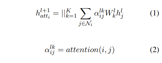
可能乍一眼看公式很多，但是其实思路还是比较简单的，比起GAT就是多考虑了关系的注意力头，计算关系得出关系权重，计算出该关系能够传来哪些特征，然后再和节点之间的注意力结果进行拼接，最后得到最终的结果。

公式（1）、（2）是GAT的计算公式。

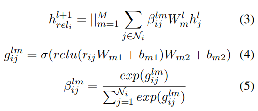
公式（3）、（4）、（5）是R-GAT中计算关系的注意力机制的部分，其中：
h_reli^l+1 为关系注意力计算后得出需要再次传来的特征
β_ij^lm 为对应关系的注意力权重
W_m^l 为对应邻居节点特征的转换矩阵参数
h_j^l 为对应邻居节点的特征

简单来说就是通过关系特征在计算出一套邻居节点的权重，然后乘以邻居节点的特征，作为原始GAT的一种补充

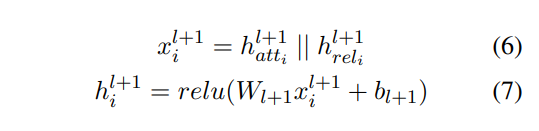
公式（6）、（7）
就是将节点的注意力权重 * 邻居节点的特征 || 关系的注意力权重 * 邻居节点的特征
再接一个全连接和激活函数，能够得到更新后的节点特征h_i^l+1

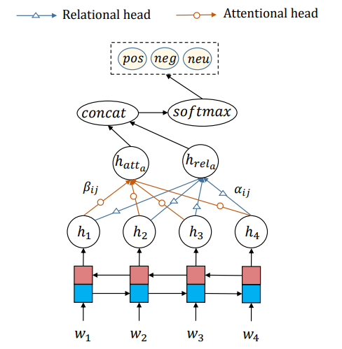
大概就是这样吧。

DGL代码实现

这个代码是从GitHub上找到的，看了一下，其实就是从DGL里封装的GATConv改过来的。

代码就只是模型的代码，并没有完整的流程代码。

阅读代码可能会有一些问题，例如消息传递、apply_edges、亦或是异构图卷积HeteroGraphConv（这些是我在阅读代码时遇到的一些问题，这个代码考虑到边的关系可能是不同类型的，因此使用了异构图卷积

还有注意力权重的计算方面，原文是拼接计算，这里是拆开分别计算，两者效果是等价的，但是后者效率较高，占用内存小。

模型构建

千言万语都在注释里了。

from dgl.nn.pytorch import HeteroGraphConv
import torch
import torch as th
import torch.nn as nn
import torch.nn.functional as F
from dgl import function as fn
from dgl.ops import edge_softmax
from dgl.utils import expand_as_pair


class GATConv(nn.Module):
    def __init__(
        self,
        in_feats, # 输入的节点特征维度
        out_feats,  # 输出的节点特征维度
        edge_feats, # 输入边的特征维度
        num_heads=1, # 注意力头数
        feat_drop=0.0, # 节点特征dropout
        attn_drop=0.0, # 注意力dropout
        edge_drop=0.0, # 边特征dropout
        negative_slope=0.2,
        activation=None,
        allow_zero_in_degree=False,
        use_symmetric_norm=False,
    ):
        super(GATConv, self).__init__()
        self._num_heads = num_heads
        self._in_src_feats, self._in_dst_feats = expand_as_pair(in_feats)
        self._out_feats = out_feats
        self._allow_zero_in_degree = allow_zero_in_degree
        self._use_symmetric_norm = use_symmetric_norm
        if isinstance(in_feats, tuple):
            self.fc_src = nn.Linear(self._in_src_feats, out_feats * num_heads, bias=False)
            self.fc_dst = nn.Linear(self._in_dst_feats, out_feats * num_heads, bias=False)
        else:
            self.fc = nn.Linear(self._in_src_feats, out_feats * num_heads, bias=False)

        self.fc_edge = nn.Linear(edge_feats, out_feats * num_heads, bias=False)

        self.attn_l = nn.Parameter(torch.FloatTensor(size=(1, num_heads, out_feats)))
        self.attn_edge=nn.Parameter(torch.FloatTensor(size=(1, num_heads, out_feats)))
        self.attn_r = nn.Parameter(torch.FloatTensor(size=(1, num_heads, out_feats)))

        self.feat_drop = nn.Dropout(feat_drop)
        self.attn_drop = nn.Dropout(attn_drop)
        self.edge_drop = edge_drop
        self.leaky_relu = nn.LeakyReLU(negative_slope)

        self.reset_parameters()
        self._activation = activation

    # 初始化参数
    def reset_parameters(self):
        gain = nn.init.calculate_gain("relu")            
        if hasattr(self, "fc"):
            nn.init.xavier_normal_(self.fc.weight, gain=gain)
        else:
            nn.init.xavier_normal_(self.fc_src.weight, gain=gain)
            nn.init.xavier_normal_(self.fc_dst.weight, gain=gain)
        nn.init.xavier_normal_(self.fc_edge.weight, gain=gain)

        nn.init.xavier_normal_(self.attn_l, gain=gain)
        nn.init.xavier_normal_(self.attn_r, gain=gain)
        nn.init.xavier_normal_(self.attn_edge, gain=gain)

    def set_allow_zero_in_degree(self, set_value):
        self._allow_zero_in_degree = set_value

    def forward(self, graph, feat):
        with graph.local_scope():
            if not self._allow_zero_in_degree:
                if (graph.in_degrees() == 0).any():
                    assert False

            # feat[0]源节点的特征        
            # feat[1]目标节点的特征
            # h_edge 边的特征
            h_src = self.feat_drop(feat[0])
            h_dst = self.feat_drop(feat[1])
            h_edge = self.feat_drop(graph.edata['feature'])


            if not hasattr(self, "fc_src"):
                self.fc_src, self.fc_dst = self.fc, self.fc
            
            # 特征赋值
            feat_src, feat_dst,feat_edge= h_src, h_dst,h_edge
            # 转换成多头注意力的形状
            feat_src = self.fc_src(h_src).view(-1, self._num_heads, self._out_feats)
            feat_dst = self.fc_dst(h_dst).view(-1, self._num_heads, self._out_feats)
            feat_edge = self.fc_edge(h_edge).view(-1, self._num_heads, self._out_feats)


            # NOTE: GAT paper uses "first concatenation then linear projection"
            # to compute attention scores, while ours is "first projection then
            # addition", the two approaches are mathematically equivalent:
            # We decompose the weight vector a mentioned in the paper into
            # [a_l || a_r], then
            # a^T [Wh_i || Wh_j] = a_l Wh_i + a_r Wh_j
            # Our implementation is much efficient because we do not need to
            # save [Wh_i || Wh_j] on edges, which is not memory-efficient. Plus,
            # addition could be optimized with DGL's built-in function u_add_v,
            # which further speeds up computation and saves memory footprint.
            # 简单来说就是拼接矩阵相乘和拆开分别矩阵相乘再相加的效果是一样的
            # 但是前者更加高效

            # 左节点的注意力权重
            el = (feat_src * self.attn_l).sum(dim=-1).unsqueeze(-1)
            graph.srcdata.update({"ft": feat_src, "el": el})
            # 右节点的注意力权重
            er = (feat_dst * self.attn_r).sum(dim=-1).unsqueeze(-1)
            graph.dstdata.update({"er": er})
            # 左节点权重+右节点权重 = 节点计算出的注意力权重（e）
            graph.apply_edges(fn.u_add_v("el", "er", "e"))

            # 边计算出来的注意力权重
            ee = (feat_edge * self.attn_edge).sum(dim=-1).unsqueeze(-1)
            # 边注意力权重加上节点注意力权重得到最终的注意力权重
            # 这里可能应该也是和那个拼接操作等价吧
            graph.edata.update({"e": graph.edata["e"]+ee})
            # 经过激活函数，一起激活和分别激活可能也是等价吧
            e = self.leaky_relu(graph.edata["e"])


            # 注意力权重的正则化
            if self.training and self.edge_drop > 0:   
                perm = torch.randperm(graph.number_of_edges(), device=graph.device)
                bound = int(graph.number_of_edges() * self.edge_drop)
                eids = perm[bound:]
                a = torch.zeros_like(e)
                a[eids] = self.attn_drop(edge_softmax(graph, e[eids], eids=eids))
                graph.edata.update({"a": a})
            else:
                graph.edata["a"] = self.attn_drop(edge_softmax(graph, e))

            # 消息传递
            graph.update_all(fn.u_mul_e("ft", "a", "m"), fn.sum("m", "ft"))
            rst = graph.dstdata["ft"]

            # 标准化
            degs = graph.in_degrees().float().clamp(min=1)
            norm = torch.pow(degs, -1)
            shp = norm.shape + (1,) * (feat_dst.dim() - 1)
            norm = torch.reshape(norm, shp)
            rst = rst * norm
            
        return rst


class RGAT(nn.Module):
   def __init__(
       self,
       in_feats, # 输入的特征维度 （边和节点一样） 
       hid_feats, # 隐藏层维度
       out_feats,  # 输出的维度
       num_heads, # 注意力头数
       rel_names, # 关系的名称（用于异构图卷积）
   ):
       super().__init__()
       self.conv1 = HeteroGraphConv({rel: GATConv(in_feats, hid_feats // num_heads, in_feats, num_heads) for rel in rel_names},aggregate='sum')
       self.conv2 = HeteroGraphConv({rel: GATConv(hid_feats, out_feats, in_feats, num_heads) for rel in rel_names},aggregate='sum')
       self.hid_feats = hid_feats

   def forward(self,graph,inputs):
       # graph 输入的异构图
       # inputs 输入节点的特征
       h = self.conv1(graph, inputs) # 第一层异构卷积
       h = {k: F.relu(v).view(-1, self.hid_feats) for k, v in h.items()} # 经过激活函数，将注意力头数拉平
       h = self.conv2(graph, h)  # 第二层异构卷积
       return h



class Model(nn.Module):
    def __init__(self, in_features, hidden_features, out_features, num_heads, rel_names):
        super().__init__()
        self.rgat = RGAT(in_features, hidden_features, out_features, num_heads, rel_names)

    def forward(self, g, x):
        h = self.rgat(g, x)
        # 输出的就是每个节点经过R-GAT后的特征
        for k, v in h.items():
           print(k, v.shape)
        return h
1
2
3
4
5
6
7
8
9
10
11
12
13
14
15
16
17
18
19
20
21
22
23
24
25
26
27
28
29
30
31
32
33
34
35
36
37
38
39
40
41
42
43
44
45
46
47
48
49
50
51
52
53
54
55
56
57
58
59
60
61
62
63
64
65
66
67
68
69
70
71
72
73
74
75
76
77
78
79
80
81
82
83
84
85
86
87
88
89
90
91
92
93
94
95
96
97
98
99
100
101
102
103
104
105
106
107
108
109
110
111
112
113
114
115
116
117
118
119
120
121
122
123
124
125
126
127
128
129
130
131
132
133
134
135
136
137
138
139
140
141
142
143
144
145
146
147
148
149
150
151
152
153
154
155
156
157
158
159
160
161
162
163
164
165
166
167
168
169
170
171
172
173
174
175
176
177
178
179
180
181
182
183
184

数据集构建

使用的是异构图，特征是随机初始化

import dgl
import torch as th
# 构建数据集测试模型
g = dgl.heterograph({
    ('user', 'follows', 'user') : ([0, 1, 2], [2, 3, 2]),
    ('user', 'plays', 'game') : ([0, 0], [1, 0]),
    ('store', 'sells', 'game')  :([0], [2])})

# 赋值边的特征
g.edges['follows'].data['feature'] = th.randn((g.number_of_edges('follows'), 2))
g.edges['plays'].data['feature'] = th.randn((g.number_of_edges('plays'), 2))
g.edges['sells'].data['feature'] = th.randn((g.number_of_edges('sells'), 2))

# 传入节点的特征
h1 = {'user' : th.randn((g.number_of_nodes('user'), 2)),
      'game' : th.randn((g.number_of_nodes('game'), 2)),
      'store' : th.randn((g.number_of_nodes('store'), 2))}
1
2
3
4
5
6
7
8
9
10
11
12
13
14
15
16
17

测试模型

# 设置输入特征为2
# 隐藏层大小为4
# 输出层大小为4
# 注意力头数为2
model = Model(2, 4, 4, 2, g.etypes)
print(model(g, h1))
1
2
3
4
5
6

输出如下：

game torch.Size([3, 2, 4])
user torch.Size([4, 2, 4])
{'game': tensor([[[0., 0., 0., 0.],
         [0., 0., 0., 0.]],

        [[0., 0., 0., 0.],
         [0., 0., 0., 0.]],

        [[0., 0., 0., 0.],
         [0., 0., 0., 0.]]], grad_fn=<SumBackward1>), 'user': tensor([[[ 0.0000,  0.0000,  0.0000,  0.0000],
         [ 0.0000,  0.0000,  0.0000,  0.0000]],

        [[ 0.0000,  0.0000,  0.0000,  0.0000],
         [ 0.0000,  0.0000,  0.0000,  0.0000]],

        [[-0.2365, -0.1838,  0.1465, -0.0919],
         [-0.0331,  0.0294,  0.0124,  0.0490]],

        [[ 0.0000,  0.0000,  0.0000,  0.0000],
         [ 0.0000,  0.0000,  0.0000,  0.0000]]], grad_fn=<SumBackward1>)}
1
2
3
4
5
6
7
8
9
10
11
12
13
14
15
16
17
18
19
20

最后输出的结果是节点的特征，维度为 节点个数 * 注意力头数 * 输出层大小。
说明测试成功。

不过模型里面的一些细节操作也不是非常确定，原文是两个注意力权重分开激活然后计算特征最后拼接转化，这里是两个权重直接求和然后一起激活，最后计算特征的，感觉好像一样，但是又感觉怪怪的，但是，大方向没错，考虑了边的注意力权重，目前还是水平有限，也不能十分确定代码是否和原文一样，有问题以后再来改吧。

算是完成前几天的任务了吧，终于结束R-GAT了！

参考

Relational Graph Attention Network for Aspect-based Sentiment Analysis
https://github.com/ChiChunxx/RGAT/blob/fb988316a0a95b6c57f24a9ea81d7d1716106ba8/model.py