2.吴恩达机器学习--逻辑回归

1. 线性可分

根据学生的两门学生成绩，预测该学生是否会被大学录取。数据集 ex2data1.txt 中包含了两门课的成绩以及是否被大学录取，0代表未录取，1代表录取。

1. 导入库，加载数据集

import matplotlib.pyplot as plt
import numpy as np
import pandas as pd

data = pd.read_csv('../data/ex2data1.txt', names=['Exam1', 'Exam2', 'Accepted'])
data.head()
1
2
3
4
5
6

2. 数据可视化扎实

fig, ax = plt.subplots()
ax.scatter(data[data['Accepted']==0]['Exam1'], data[data['Accepted']==0]['Exam2'], c='r', marker='x', label='y=0')
ax.scatter(data[data['Accepted']==1]['Exam1'], data[data['Accepted']==1]['Exam2'], c='b', marker='o', label='y=1')
ax.legend()
ax.set(xlabel='exam1', ylabel='exam2')
plt.show()
1
2
3
4
5
6

3. 构造数据集

# 与线性回归做法一致
def get_Xy(data):
    data.insert(0, 'ones', 1)
    X_ = data.iloc[:, 0:-1]
    X = X_.values
    
    y_ = data.iloc[:, -1]
    y = y_.values.reshape(len(y_), 1)
    
    return X, y

X, y = get_Xy(data)
1
2
3
4
5
6
7
8
9
10
11
12

4. 定义sigmoid函数和损失函数

  对于逻辑回归模型，我们构建的模型为：$$P(y=1|x;\theta )=\frac{1}{1+e^{-{\theta }^{T}x}}$$
  代码中（$m$表示样本维度，$n$表示样本个数）： X = [ 1 x 01 x 02 ⋯ x 0 m 1 x 11 x 12 ⋯ x 1 m ⋮ ⋮ ⋮ ⋮ 1 x n 1 x n 2 ⋯ x n m ] , θ = [ θ 0 θ 1 ⋮ θ m ] X=

, \theta= X=⎣⎢⎢⎢⎡​11⋮1​x01​x11​⋮xn1​​x02​x12​⋮xn2​​⋯⋯⋮⋯​x0m​x1m​xnm​​⎦⎥⎥⎥⎤​,θ=⎣⎢⎢⎢⎡​θ0​θ1​⋮θm​​⎦⎥⎥⎥⎤​
  所以在实际实现中，是直接用$X$与$\theta$做内积。
  在模型的数学形式确定后，剩下的就是如何去求解模型中的参数 $\theta$。而在已知模型和一定样本的情况下，估计模型的参数，在统计学中常用的是极大似然估计方法。即找到一组参数 $\theta$，使得在这组参数下，样本数据的似然度（概率）最大。
  对于逻辑回归模型，假定的概率分布是伯努利分布，根据伯努利分布的定义，其概率质量函数$PMF$为： P ( X = n ) = { 1 − p n = 0 p n = 1 P(X = n) =\left\{

1−ppn=0n=1$$\begin{array}{rcl}1-p& & n=0\\ p& & n=1\end{array}$$

\right. P(X=n)={1−pp​​n=0n=1​
  所以似然函数可以写成：$$L(\theta )=\prod _{i=1}^{m}P(y=1|x_i{)}^{y_i}P(y=0|x_i{)}^{1-y_i}$$
  对数似然函数则为：$$\ln L(\theta )=\sum _{i=1}^m[y_i\ln P(y=1|x_i)+(1-y_i)\ln P(y=0|x_i)]$$$$\ln L(\theta )=\sum _{i=1}^m[y_i\ln P(y=1|x_i)+(1-y_i)\ln (1-P(y=1|x_i))]$$
  由于在机器学习中，我们通常是对代价函数做最小化处理，所以最大化似然函数，可以在似然函数前面加个负号形成代价函数，从而转换为最小化化代价函数：$$cost(y,p(y|x))=-\frac{1}{m}\sum _{i=1}^m[y_i\ln P(y=1|x_i)+(1-y_i)\ln (1-P(y=1|x_i))]$$

def sigmoid(z):
    return 1 / (1 + np.exp(-z))

def costFunction(X, y, theta):
    return -np.sum(y * np.log(sigmoid(X @ theta)) + (1 - y) * np.log(1 - sigmoid(X @ theta))) / len(X)
1
2
3
4
5

5. 初始化参数

theta = np.zeros((3, 1))
cost_init = costFunction(X, y, theta)
cost_init
1
2
3

  此时求得的初始化损失值为：0.6931471805599453

6. 定义梯度下降函数

  损失函数关于$\theta$的偏导数为：$${\theta }_j:={\theta }_j-\alpha \frac{\partial }{\partial {\theta }_j}J(\theta )$$
$$\frac{\partial }{\partial {\theta }_j}J(\theta )=\frac{1}{m}\sum _{i=1}^m(h_{\theta }(x_i)-y_i)x_{ij}$$

# 梯度下降函数
def gradientDescent(X, y, theta, iters, alpha):
    m = len(X)
    costs = []
    
    for i in range(iters):
        A = sigmoid(X @ theta)
        theta = theta - alpha * X.T @ (A - y) / m
        cost = costFunction(X, y, theta)
        costs.append(cost)
        
        if i % 100 == 0:
            print(f'迭代次数i={i}，损失函数值cost={cost}')
    return costs, theta
1
2
3
4
5
6
7
8
9
10
11
12
13
14

7. 执行梯度下降函数，获取最佳参数

alpha = 0.004
iters = 200000

costs, theta_final = gradientDescent(X, y, theta, iters, alpha)
theta_final
1
2
3
4
5

  经过计算可得最佳参数为：array([[-23.77446812], [0.20684452], [0.19996036]])

8. 预测及准确率

def predict(X, theta):
    prob = sigmoid(X @ theta)
    return [1 if x >= 0.5 else 0 for x in prob

y_ = np.array(predict(X, theta_final))
y_pre = y_.reshape(len(y_), 1)

acc = np.mean(y_pre == y)
acc
1
2
3
4
5
6
7
8
9

  所得模型的准确率为：0.91

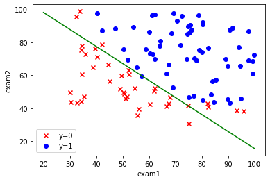
9. 可视化展示

  由假设的模型可知，${\theta }^{T}X=0$ 为两类别的分界线，即 ${\theta }_0+{\theta }_1{x}_1+{\theta }_2{x}_2=0$。由此，可根据 $x_1$ 计算出 $x_2$ 的值，即得到 $x_2$ 关于 $x_1$ 的函数：$$x_2=-\frac{{\theta }_0}{{\theta }_2}-\frac{{\theta }_1}{{\theta }_2}{x}_1$$

coef1 = -theta_final[0, 0] / theta_final[2, 0]
coef2 = -theta_final[1, 0] / theta_final[2, 0]

x1 = np.linspace(20, 100, 100)
x2 = coef1 + coef2 * x1

fig,ax = plt.subplots()
ax.scatter(data[data['Accepted']==0]['Exam1'],data[data['Accepted']==0]['Exam2'],c='r',marker='x',label='y=0')
ax.scatter(data[data['Accepted']==1]['Exam1'],data[data['Accepted']==1]['Exam2'],c='b',marker='o',label='y=1')
ax.legend()
ax.set(xlabel='exam1',
          ylabel='exam2')

ax.plot(x1,x2,c='g')
plt.show()
1
2
3
4
5
6
7
8
9
10
11
12
13
14
15

2. 线性不可分

设想你是工厂的生产主管，你要决定是否芯片要被接受或抛弃。ex2data2.txt是芯片在两次测试中的结果。

1. 读取数据并进行可视化展示

data = pd.read_csv('../data/ex2data2.txt', names=['Test1', 'Test2', 'Accepted'])
data.head()

fig, ax = plt.subplots()
ax.scatter(data[data['Accepted']==0]['Test1'],data[data['Accepted']==0]['Test2'],c='r',marker='x',label='y=0')
ax.scatter(data[data['Accepted']==1]['Test1'],data[data['Accepted']==1]['Test2'],c='b',marker='o',label='y=1')
ax.legend()
ax.set(xlabel='Test1', ylabel='Test2')
plt.show()
1
2
3
4
5
6
7
8
9

2. 特征映射

  当逻辑回归问题较复杂，原始特征不足以支持构建模型时，可以通过组合原始特征成为多项式，创建更多特征，使得决策边界呈现高阶函数的形状，从而适应复杂的分类问题。

# 特征映射：共映射到(power+1)*(power+2)/2个特征
def feature_mapping(x1, x2, power):
    data = {}
    
    for i in np.arange(power + 1):
        for j in np.arange(i + 1):
            data['F{}{}'.format(i-j, j)] = np.power(x1, i-j) * np.power(x2, j)
    return pd.DataFrame(data)

x1 = data['Test1']
x2 = data['Test2']
data2 = feature_mapping(x1, x2, 6)
data2.head()
1
2
3
4
5
6
7
8
9
10
11
12
13

3. 构造数据集

X = data2.values
y = data.iloc[:, -1].values.reshape(len(X), 1)
1
2

4. 定义sigmoid函数和损失函数

  算法没有很好的拟合训练集，称为欠拟合或高偏差。算法有很强的偏见，罔顾数据的不符，先入为主地拟合一条直线，最终导致拟合训练集效果很差。
  算法过度拟合数据集，称为过拟合或高方差（变量数量多，高阶项太多）。它无法泛化到新的样本中。泛化指的是模型应用到新样本的能力。
  下图中依次是：低偏差低方差，低偏差高方差，高偏差低方差，高偏差高方差

  解决过拟合，要么减少特征变量的数量，要么使用正则化。但是舍弃特征变量的缺点是，同时舍弃了关于问题的一些信息，我们可能不想舍弃。所以我们接下来使用正则化，保留所有的特征变量，但是减小量级或者限制 $\theta$ 的大小。
  如图所示，在原有的需要最小化的代价函数的基础上，添加了 $1000{\theta }_3^2+1000{\theta }_4^2$ 两项，称为惩罚项。

  现在我们想要 $J$ 尽可能小，就是要 ${\theta }_3$ 和 ${\theta }_4$ 尽可能小，尽量接近0，就像我们去掉了 ${\theta }_3$ 和 ${\theta }_4$，那么我们这个高阶项就近乎没有了。
  正则化思想是参数值较小意味着更简单的假设模型，一般来说， $\theta$ 的值越小，我们得到的曲线越平滑，也越简单，更不容易出现过拟合。
  由于我们并不知道哪个参数该减小，所以我们选择惩罚所有参数，缩小每一个 ${\theta }_j$ 的值除了 ${\theta }_0$ ，因为 $x_0^{(i)}=1$ ，正则化后的损失函数为：
$$cost(y,p(y|x))=-\frac{1}{m}\sum _{i=1}^m[y_i\ln P(y=1|x_i)+(1-y_i)\ln (1-P(y=1|x_i))]+\frac{\lambda }{2m}\sum _{j=1}^m{\theta }_j^2$$
  正则化系数 $\lambda$ 控制两个目标之间的取舍：第一个目标是第一项，我们想更好地拟合数据，希望第一项尽可能小；第二个目标与正则化系数有关，我们要保持参数尽可能小，保持模型的相对简单，避免过拟合。 $\lambda$ 控制这两个目标的平衡关系，过小则惩罚力度不够导致过拟合，过大则所有参数为0导致欠拟合。
  梯度下降的过程为：

def sigmoid(z):
    return 1 / (1 + np.exp(-z))
    
def costFunction(X, y, theta, lamda):
    A = sigmoid(X @ theta)
    m = len(X)
    
    cost = -np.sum(y * np.log(A) + (1 - y) * np.log(1 - A)) / m
    reg = np.sum(np.power(theta[1:], 2)) * lamda / (2 * m)
    
    return cost + reg
1
2
3
4
5
6
7
8
9
10
11

5. 初始化参数

theta = np.zeros((28, 1))
lamda = 1

cost_init = costFunction(X, y, theta, lamda)
cost_init
1
2
3
4
5

  得到的初始损失值为：0.6931471805599454

6. 定义梯度下降函数

def gradientDescent(X, y, theta, alpha, iters, lamda):
    costs = []
    m= len(X)
    
    for i in range(iters):
        reg = theta[1:] * lamda / m
        reg = np.insert(reg, 0, values=0, axis=0)
        
        theta = theta - (X.T @ (sigmoid(X @ theta) - y)) / m - reg
        cost = costFunction(X, y, theta, lamda)
        costs.append(cost)
        
        if i % 1000 == 0:
            print(f'迭代次数i={i}，损失函数值cost={cost}')
            
    return theta, costs
1
2
3
4
5
6
7
8
9
10
11
12
13
14
15
16

7. 寻找最佳参数

alpha = 0.001
iters = 200000
lamda = 0.1

theta_final, costs = gradientDescent(X, y, theta, alpha, iters, lamda)
1
2
3
4
5

8. 预测，计算准确率

def predict(X, theta):
    prob = sigmoid(X @ theta)
    return [1 if x >= 0.5 else 0 for x in prob]

y_ = np.array(predict(X, theta_final))
y_pre = y_.reshape(len(y_), 1)

acc = np.mean(y_pre == y)
acc
1
2
3
4
5
6
7
8
9

  得到的准确率为：0.8389830508474576

9. 可视化展示

x = np.linspace(-1.2,1.2,200)
xx,yy = np.meshgrid(x,x)
z = feature_mapping(xx.ravel(),yy.ravel(),6).values

zz = z @ theta_final
zz = zz.reshape(xx.shape)

fig,ax = plt.subplots()
ax.scatter(data[data['Accepted']==0]['Test1'],data[data['Accepted']==0]['Test2'],c='r',marker='x',label='y=0')
ax.scatter(data[data['Accepted']==1]['Test1'],data[data['Accepted']==1]['Test2'],c='b',marker='o',label='y=1')
ax.legend()
ax.set(xlabel='Test1', ylabel='Test2')

plt.contour(xx,yy,zz,0)
plt.show()
1
2
3
4
5
6
7
8
9
10
11
12
13
14
15