Graphs and where to find them

Attributes of graphs

图的属性: 结点、边、全局属性

图的属性可由 Embedding 向量表示

• 每个结点和边的信息都可以由一个 Embedding 向量表示。全局信息也可以由一个 Embedding 向量表示
  

Images as graphs

Text as graphs

Of course, in practice, this is not usually how text and images are encoded: these graph representations are redundant since all images and all text will have very regular structures. For instance, images have a banded structure in their adjacency matrix because all nodes (pixels) are connected in a grid. The adjacency matrix for text is just a diagonal line, because each word only connects to the prior word, and to the next one.

Graph-valued data in the wild

Molecules as graphs

Social networks as graphs

What types of problems have graph structured data?

Graph-level task

• 在 Graph-level task 中，我们的主要目标是预测整个图的属性。例如将一个分子表示成一个图，然后预测该分子是否含有两个环
  

Node-level task

• 在 Node-level task 中，主要目标是预测图中结点的属性 (identity or role)。例如在下面的社交网络图中，John A 和 Mr. Hi 决裂了，要求预测每个人更支持谁
  

Edge-level task

• 在 Edge-level task 中，主要目标是预测图中边的属性。例如在下面的图中，使用语义分割将人物和背景分开作为不同结点，然后要求预测人物之间的关系，也就是预测边的属性 (image scene understanding)
  

The challenges of using graphs in machine learning

• 使用神经网络解决图问题首先需要一个合适的方法对图的信息进行表示。图有四种信息：结点、边、全局信息和连通性
• 前面提到，结点、边和全局信息可以由 Embedding 向量进行表示，但连通性的表示就没那么容易了。对于连通性的表示，最简单的方法是使用邻接矩阵，但当图的结点数很多时，邻接矩阵会变得非常稀疏，在空间上比较低效。此外，对于同一张图，有很多等价的邻接矩阵，我们无法保证神经网络在输入这些不同的等价邻接矩阵时还能输出相同的结果 (that is to say, they are not permutation invariant). 一种更加优雅和存储高效的表示方法是邻接列表 (adjacency lists)，它将每条从结点 $n_i$ 指向结点 $n_j$ 的边都表示为一个二元组 $(i,j)$ (permutation invariant)
  

上图中，结点、边和全局信息都只用了一个标量表示，但更实际的方法是用向量表示

Graph Neural Networks

• A GNN is an optimizable transformation on all attributes of the graph (nodes, edges, global-context) that preserves graph symmetries (permutation invariances).

下面我们将使用 “message passing neural network” (信息传递网络) 框架来构建 GNN.

The simplest GNN

• 下面先介绍最简单的 GNN，它暂时不考虑图的连通性信息，也就不能利用图的结构信息

---

GNN layer / GNN block

• GNN 采取了 “graph-in, graph-out” 的架构，模型输入一张图，然后通过不断对图的结点、边以及全局信息的 Embedding 向量进行变换 (不改变输入图的连通性) 来得到最终的预测
• GNN 层对结点向量、边向量和全局向量分别构造 3 个 MLP，最终得到 3 个相同维度的 Embedding 向量
  

As is common with neural networks modules or layers, we can stack these GNN layers together.

GNN Predictions by Pooling Information

下面讲解 GNN 的最后一层如何得到预测值

• 先考虑一个最简单的情况。如果要对图的所有结点进行多分类，那么直接用一个 MLP 将最终的结点向量变换到指定维度然后接 Softmax 就行了
  如果我们只有边的信息而没有结点信息，那么我们也就没有结点的 Embedding 向量。此时如果想要对结点进行预测，可以通过 pooling ${\rho }_{E_n\to V_n}$ 来由边信息得到结点信息，也就是将结点邻接的边的向量和全局向量加起来当作结点向量 (如果结点向量和边向量维度不一样，那么可以在 pooling 之前先对边向量进行投影再相加，也可以 concat 之后再进行投影)
  如果只有结点向量没有边向量，想要对边进行预测，那么分类部分的网络结构如下：
  如果只有结点向量，想要对整个图进行预测，那么类似 Global Average Pooling，我们可以汇集所有结点信息进行预测：
  

---

An end-to-end prediction task with a GNN model

GCN: Passing messages between parts of the graph

下面将介绍 GNN 如何利用图的结构信息 (连通性)

• 在 GNN layer 中，我们也可以利用 pooling 来进行相邻结点或相邻边之间的信息传递 (Message passing)。以结点为例，GNN layer 的输出结点向量为输入结点向量及其相邻结点向量相加后经过 MLP 得到 (the simplest type of message-passing GNN layer)
  

上述的 message-passing 其实和卷积有些相似，因此带信息汇聚的 GNN 也被称为 GCN (图卷积神经网络)。如果将结点看作像素点，相邻结点看作同一个卷积核作用的区域，那么 message-passing 就相当于用一个数值全为 1 的卷积核进行卷积。类似于多个卷积层可以增加感受野，多个 GNN 层的堆叠也可以使得生成的结点/边向量包含很多结点/边的信息

Learning edge representations

• 之前讲到，在做预测时，如果某些属性缺失，就需要在最后一层利用 pooling 从别的属性进行信息汇聚，但实际上我们可以使用 message passing 在 GNN 层更早地进行结点和边之间的信息汇聚

---

• 如下图所示，我们可以先进行结点到边的 pooling，再使用更新过的边向量进行边到结点的 pooling
  当然也可以先进行边到结点的 pooling，再使用更新过的结点向量进行结点到边的 pooling：
  甚至可以兼而有之，用一种 “编织” 形式 (‘weave’ fashion) 进行更新，它包含 4 个变换: node to node (linear), edge to edge (linear), node to edge (edge layer), edge to node (node layer)：
  

Adding global representations

• 目前为止介绍的 GNN 只在结点和边之间进行了消息传递而没有用到全局信息，因此有一个缺陷：如果只在结点和边之间进行了消息传递，那么当图大且稀疏时，消息从一个结点传递到另一个点就需要经过很多个 GNN 层。为此，我们需要加入全局信息，也被称作 master node 或 context vector。可以将全局向量看作一个连接所有边和结点的虚拟结点，用于在所有边和结点之间传递消息
• 在引入全局向量后，GNN 层的信息融合可由下图表示，依次进行边向量、结点向量、全局向量的更新：
  
• 通过上述方法得到的每个图属性对应向量都包含了全图的信息，因此在最后预测时，我们可以利用 pooling 来对信息进行充分融合。例如当对一个结点进行预测时，我们可以融合它的邻接结点、邻接边以及全局信息 (可以选择不同的融合方式，例如连接后映射；映射后相加；feature-wise modulation layer…)
  

GNN playground

• 在文章 A Gentle Introduction to Graph Neural Networks 中，作者做了一个比较小的分子图预测数据集 (一个二分类 graph-level prediction task)，并把 GNN 的训练程序嵌入到了 JavaScript 中便于调节超参数，最后还做了很多对比实验来探究不同超参数对 GNN 模型的影响

---

分子预测任务

• 在分子预测任务中，结点为 Carbon, Nitrogen, Oxygen, Fluorine 中的一种，边为 single, double, triple, aromatic 中的一种，因此结点和边均为 one-hot encodings；模型结构为若干个 GNN 层的堆叠，最后用线性层接 Sigmoid 进行二分类 (GNN 层中的 MLP 为 1 层 MLP + ReLU + Layer norm)
  

Node/Edge/Global embedding 旁的对勾代表是否 Node/Edge/Global embedding 是否进行消息传递；图中的可视化是通过对 GNN 的 penultimate layer activations 进行 PCA 降维后得到的，圆圈的填充色代表预测值，边框色代表真值

---

Some empirical GNN design lessons

• 参数量：参数量与模型性能正相关。同时也可以注意到，只要选取较好的超参数，使用较少的参数也可以得到比较好的结果
  

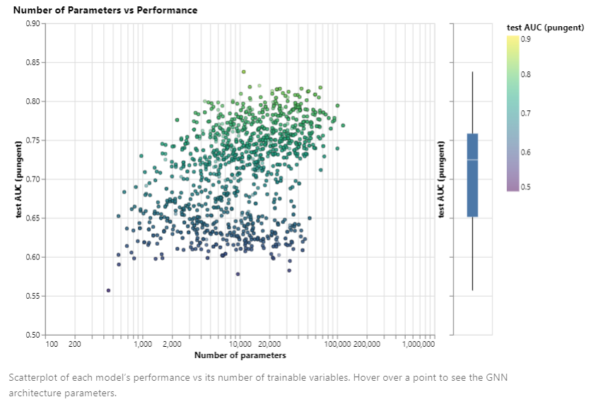
图中的每个点都代表了使用某种超参的模型。$x$ 轴代表模型参数量，$y$ 轴代表 AUC

• Embedding 维数：We can notice that models with higher dimensionality tend to have better mean and lower bound performance but the same trend is not found for the maximum. Some of the top-performing models can be found for smaller dimensions.
  
• GNN 层数：The box plot shows a similar trend, while the mean performance tends to increase with the number of layers, the best performing models do not have three or four layers, but two. Furthermore, the lower bound for performance decreases with four layers. This effect has been observed before, GNN with a higher number of layers will broadcast information at a higher distance and can risk having their node representations ‘diluted’ from many successive iterations
  
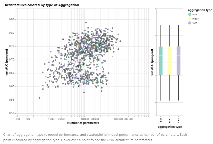
• 信息聚合方式：在这个数据集上，聚合方式对模型性能影响不大
  
• 消息传递的方式：总体而言，消息传递时使用的图属性越多，模型性能越好
  

Final thoughts

• 图是一种强大且丰富的结构化数据类型，但图也存在一些缺陷。例如在图上做优化是非常难的 (稀疏的架构，动态的结构)，这使得如何使 GNN 高效地运行在 CPU、GPU 上成为了一个非常难的任务；同时 GNN 对超参数非常敏感。这些因素导致 GNN 门槛较高，当前工业界应用较少

References

• 零基础多图详解图神经网络（GNN/GCN）【论文精读】
• A Gentle Introduction to Graph Neural Networks
• more: Understanding Convolutions on Graphs (how convolutions over images generalize naturally to convolutions over graphs), Into the Weeds