-
Central Limit Theorem
The central limit theorem is an often quoted, but misunderstood pillar from statistics and machine learning.it has important implications about how and why we can make inferences about the skill of machine learning models, such as whether one model is statistically better than another and confidence intervals on models skill.In this tutorial, you will discover the central limit theorem and the implications of this important pillar of statistics and probability on applied machine learning. After completing this tutorial, you will know:
- The central limit theorem describes the shape of the distribution of sample means as a Gaussian, which is a distribution that statistics knows a lot about.
- How to develop an example of simulated dice rolls in Python to demonstrate the central limit theorem.
- How the central limit theorem and knowledge of the Gaussian distribution is used to make inferences about model performance in applied machine learning.
1.2 Centrol Limit Theorem
The Central Limit Theorem, or CLT for short, is an important finding and pillar in the fields of statistics and probability. It may seem a little esoteric at first, so hang in there. It turns out that the finding is critically important for making inferences in applied machine learning.
The theorem states that as the size of the sample increases, the distribution of the mean across multiple samples will approximate a Gaussian distribution. Let’s break this down.
We can imagine performing a trial and getting a result or an observation. We can repeat the trial again and get a new independent observation. Collected together, multiple observations represents a sample of observations. A sample is a group of observations from a broader population of all possible observations that could be made given trials.
- Observation: Result from one trial of an experiment.
- Sample: Group of results gathered from separate independent trials.
- Population: Space of all possible observations that could be seen from a trial.
Firstly, the central limit theorem is impressive, especially as this will occur no matter the shape of the population distribution from which we are drawing samples. It demonstrates that the distribution of errors from estimating the population mean fit a distribution that the field of statistics knows a lot about. Secondly, this estimate of the Gaussian distribution will be more accurate as the size of the samples drawn from the population is increased. This means that if we use our knowledge of the Gaussian distribution in general to start making inferences about the means of samples drawn from a population, that these inferences will become more useful as we increase our sample size.
One interesting implication of the central limit theorem mentioned to me one time by a very clever scientist is that you can use it to generate Gaussian random numbers. You can generate uniformly random integers, sum groups of them together, and the results of the sums will be Gaussian. Remember that the mean is just the normalized sum of the sample. It’s a slower method for generating random Gaussian variables than other methods (like the Box-Muller method), but a clear (and clever) application of the theorem.
1.2.1 Law of Large Numbers
The central limit theorem is often confused with the law of large numbers by beginners. The law of large numbers is another different theorem from statistics. It is simpler in that it states that as the size of a sample is increased, the more accurate of an estimate the sample mean will be of the population mean. The central limit theorem does not state anything about a single sample mean; instead, it is broader and states something about the shape or the distribution of sample means.
The law of large numbers is intuitive. It is why we think that collecting more data will lead to a more representative sample of observations from the domain. The theorem supports this intuition. The central limit theorem is not intuitive. Instead, it is a finding that we can exploit in order to make claims about sample means.
1.3 Worked Example with Dice
We can make the central limit theorem concrete with a worked example involving the rolling of die. Remember that a die is a cube with a different number on each side from 1-to-6. Each number has a 1-in-6 likelihood to turn up from a roll. The distribution of the numbers that turn up from a dice roll is uniform given the equal likelihood. We can use the randint() NumPy function to generate a specific number of random dice rolls (e.g. 50) between 1 and 6.
- # Example of How to simulate dice rolls
- # generate a sample of die rolls
- rolls = randint(1, 7, 50)
The complete example is listed below.
- # generate random dice rolls
- from numpy.random import seed
- from numpy.random import randint
- from numpy import mean
- # seed the random number generator
- seed(1)
- # generate a sample of die rolls
- rolls = randint(1, 7, 50)
- print(rolls)
- print(mean(rolls))
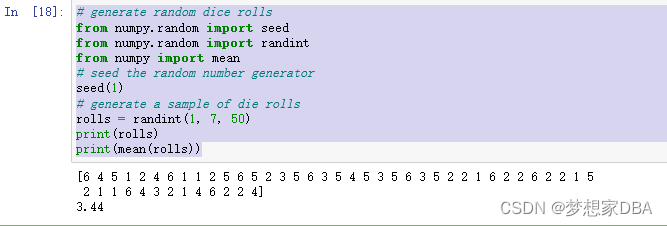
Running the example generates and prints the sample of 50 die rolls and the mean value of the sample. We know that the mean value of the distribution is 3.5 calculated as 1+2+3+4+5+6/ 6 or 21/6 . We can see that the mean of the sample is slightly wrong, which is to be expected because it is an estimate of the population mean.

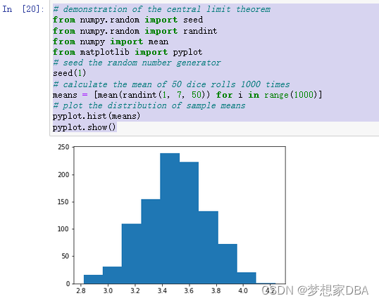
This is the result of rolling the simulated die 50 times. We can then repeat this process multiple times, such as 1,000. This will give us a result of 1,000 sample means. According to the central limit theorem, the distribution of these sample means will be Gaussian. The example below performs this experiment and plots the resulting distribution of sample means.
- # demonstration of the central limit theorem
- from numpy.random import seed
- from numpy.random import randint
- from numpy import mean
- from matplotlib import pyplot
- # seed the random number generator
- seed(1)
- # calculate the mean of 50 dice rolls 1000 times
- means = [mean(randint(1, 7, 50)) for i in range(1000)]
- # plot the distribution of sample means
- pyplot.hist(means)
- pyplot.show()
Running the example creates a histogram plot of the sample means. We can tell from the shape of the distribution that the distribution is Gaussian. It’s interesting to note the amount of error in the sample mean that we can see in 1,000 trials of 50 dice rolls. Further, the central limit theorem also states that as the size of each sample, in this case 50, is increased, then the better the sample means will approximate a Gaussian distribution.

1.4 Impact on Machine Learning
The central limit theorem has important implications in applied machine learning. The theorem does inform the solution to linear algorithms such as linear regression, but not exotic methods like artificial neural networks that are solved using numerical optimization methods. Instead, we must use experiments to observe and record the behavior of the algorithms and use statistical methods to interpret their results. Let’s look at two important examples.
1.4.1 Significance Tests
In order to make inferences about the skill of a model compared to the skill of another model, we must use tools such as statistical significance tests.
The ability to make inference claims like this is due to the central limit theorem and our knowledge of the Gaussian distribution and how likely the two sample means are to be a part of the same Gaussian distribution of sample means.
1.4.2 Confidence Intervals(置信区间)
Once we have trained a final model, we may wish to make an inference about how skillful the model is expected to be in practice. The presentation of this uncertainty is called a confidence interval. We can develop multiple independent (or close to independent) evaluations of a model accuracy to result in a population of candidate skill estimates. The mean of these skill estimates will be an estimate (with error) of the true underlying estimate of the model skill on the problem. With knowledge that the sample mean will be a part of a Gaussian distribution from the central limit theorem, we can use knowledge of the Gaussian distribution to estimate the likelihood of the sample mean based on the sample size and calculate an interval of desired confidence around the skill of the model.
-
相关阅读:
Pycharm连接远程服务器 导入远程包时本地显示红色解决方法
Hive 表 DML 操作——Hive 表 DML 操作——第1关:将文件中的数据导入(Load)到 Hive 表中
Linux常用命令——grep命令
【Python】python入门(一):JupyterLab安装、使用
论文综述的重要性及写作
【网络编程】进程间的通信
Sprinig Boot优雅实现接口幂等性
Java27岁了——我与Java初识
华中科技大学机试大位数加法器C语言编程解答
12家硬件厂商发布飞桨生态发行版 软硬一体协同发展
- 原文地址:https://blog.csdn.net/u011868279/article/details/125471137