-
Law of Large Numbers
In this tutorial, you will discover the law of large numbers and why it is important in applied machine learning. After completing this tutorial, you will know:
- The law of large numbers supports the intuition that the sample becomes more representative of the population as its size is increased.
- How to develop a small example in Python to demonstrate the decrease in error from the increase in sample size.
- The law of large numbers is critical for understanding the selction of training datasets, test datasets, and in the evaluation of model skill in machine learning.
1.1 Law of Large Numbers
The law of large numbers is a theorem from probability and statistics that suggests that the average result from repeating an experiment multiple times will better approximate the true or expected underlying result.
The standalone and independent repetition of the experiment will perform multiple trials and lead to multiple observations. All sample observations for an experiment are drawn from an idealized population of observations.
- Observation: Result from one trial of an experiment
- Sample: Group of results gathered from separate independent trails.
- Population: Space of all possible observations that could be seen from a trial.
1.1.1 Independent and Identically Distributed
It is important to be clear that the observations in the sample must be independent.This means that the trial is run in an identical manner and does not depend on the results of any other trial. This is often reasonable and easy to achieve in computers, although can be difficult elsewhere (e.g. how do you achieve identically random rolls of a dice?). In statistics, this expectation is called independent and identically distributed, or IID, iid, or i.i.d. for short. This is to ensure that the samples are indeed drawn from the same underlying population distribution.
1.1.2 Regression to the Mean
The law of large numbers helps us understand why we cannot trust a single observation from an experiment in isolation. We expect that a single result or the mean result from a small sample is likely. That is close to the central tendency, the mean of the population distribution. It may not be; in fact, it may be very strange or unlikely. The law reminds us to repeat the experiment in order to develop a large and representative sample of observations before we start making inferences about what the result means. As we increase the sample size, the finding or mean of the sample will move back toward the population mean, back toward the true underlying expected value. This is called regression to the mean or sometimes reversion to the mean. It is why we must be skeptical of inferences from small sample sizes, called small n.
1.1.3 Law of Truly Large Numbers
Related to the regression to the mean is the idea of the law of truly large numbers. This is the idea that when we start investigating or working with extremely large samples of observations, we increase the likelihood of seeing something strange. That by having so many samples of the underlying population distribution, the sample will contain some astronomically rare events. Again, we must be wary not to make inferences from single cases. This is especially important to consider when running queries and investigating big data.
1.2 Worked Example
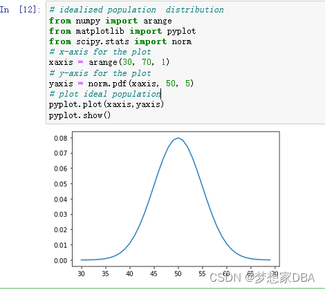
We can demonstrate the law of large numbers with a small worked example. First, we can design an idealized underlying distribution. We will use a Gaussian distribution with a mean of 50 and a standard deviation of 5. The expected value or mean of this population is therefore 50. Below is some code that generates a plot of this idealized distribution.
- # idealized population distribution
- from numpy import arange
- from matplotlib import pyplot
- from scipy.stats import norm
- # x-axis for the plot
- xaxis = arange(30, 70, 1)
- # y-axis for the plot
- yaxis = norm.pdf(xaxis, 50, 5)
- # plot ideal population
- pyplot.plot(xaxis,yaxis)
- pyplot.show()
Running the code creates a plot of the designed population with the familiar bell shape.

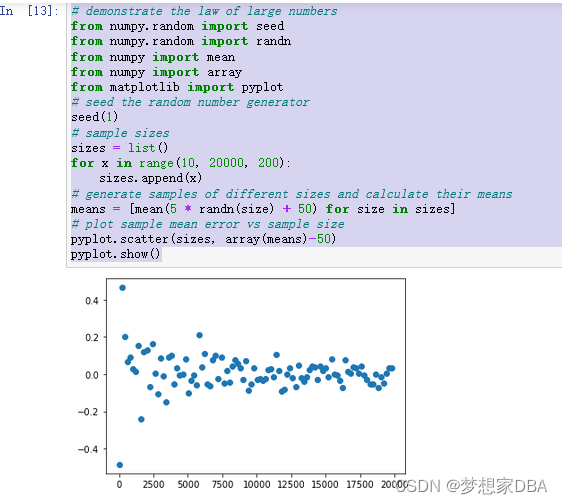
The example below calculates samples of different sizes, estimates the mean and plots the errors in the mean from the expected mean (50).
- # demonstrate the law of large numbers
- from numpy.random import seed
- from numpy.random import randn
- from numpy import mean
- from numpy import array
- from matplotlib import pyplot
- # seed the random number generator
- seed(1)
- # sample sizes
- sizes = list()
- for x in range(10, 20000, 200):
- sizes.append(x)
- # generate samples of different sizes and calculate their means
- means = [mean(5 * randn(size) + 50) for size in sizes]
- # plot sample mean error vs sample size
- pyplot.scatter(sizes, array(means)-50)
- pyplot.show()
Running the example creates a plot that compares the size of the sample to the error of the sample mean from the population mean. Generally, we can see that larger sample sizes have less error, and we would expect this trend to continue, on average. We can also see that some sample means overestimate and some underestimate. Do not fall into the trap of assuming that the underestimate will fall on one side or another.

1.3 Implications in Machine Learning
The law of large numbers has important implications in applied machine learning. Let’s take a moment to highlight a few of these implications.
1.3.1 Training Data
The data used to train the model must be representative of the observations from the domain. This really means that it must contain enough information to generalize to the true unknown and underlying distribution of the population.
Keep this in mind during data collection, data cleaning, and data preparation. You may choose to exclude sections of the underlying population by setting hard limits on observed values (e.g. for outliers) where you expect data to be too sparse to model effectively.
1.3.2 Test Data
The thoughts given to the training dataset must also be given to the test dataset. This is often neglected with the blind use of 80/20 spits for train/test data or the blind use of 10-fold cross-validation, even on datasets where the size of 1/10th of the available data may not be a suitable representative of observations from the problem domain.
1.3.3 Model Skill Evaluation
Consider the law of large numbers when presenting the estimated skill of a model on unseen data. It provides a defense for not simply reporting or proceeding with a model based on a skill score from a single train/test evaluation. It highlights the need to develop a sample of multiple independent (or close to independent) evaluations of a given model such that the mean reported skill from the sample is an accurate enough estimate of population mean.
-
相关阅读:
电影数据读取、分析与展示(Python+Scrapy)
美国服务器速度变慢了有没有解决办法?
node.js+室内装修风格选择系统 毕业设计-附源码211552
oracle19c单机应用补丁-缺少包导致失败
静态/动态代理模式
【python】1.python3.12.2和pycharm社区版的安装指南
【云原生】Docker 进阶 -- 阿里云服务器安装Docker Compose与初体验
Leet code 179 最大数
安装mysql
字节跳动的顶级架构师竟然整理出程序员向架构师的必备转型之路
- 原文地址:https://blog.csdn.net/u011868279/article/details/125470019