GDP与人预期寿命的关系图----R

单位GDP与寿命的关系统计绘图

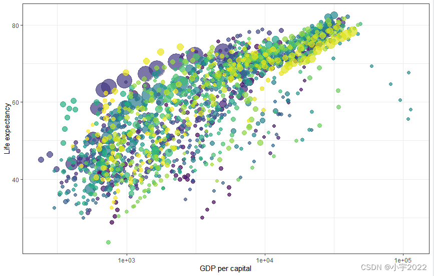
library(ggplot2)
library(gganimate)
theme_set(theme_bw())
library(gapminder)
head(gapminder)
p <- ggplot(
  gapminder, 
  aes(x = gdpPercap, y=lifeExp, size = pop, colour = country)
) +
  geom_point(show.legend = FALSE, alpha = 0.7) +
  scale_color_viridis_d() +
  scale_size(range = c(2, 12)) +
  scale_x_log10() +
  labs(x = "GDP per capital", y = "Life expectancy")
p
1
2
3
4
5
6
7
8
9
10
11
12
13
14
15

通过不同州的时间数据进行转换

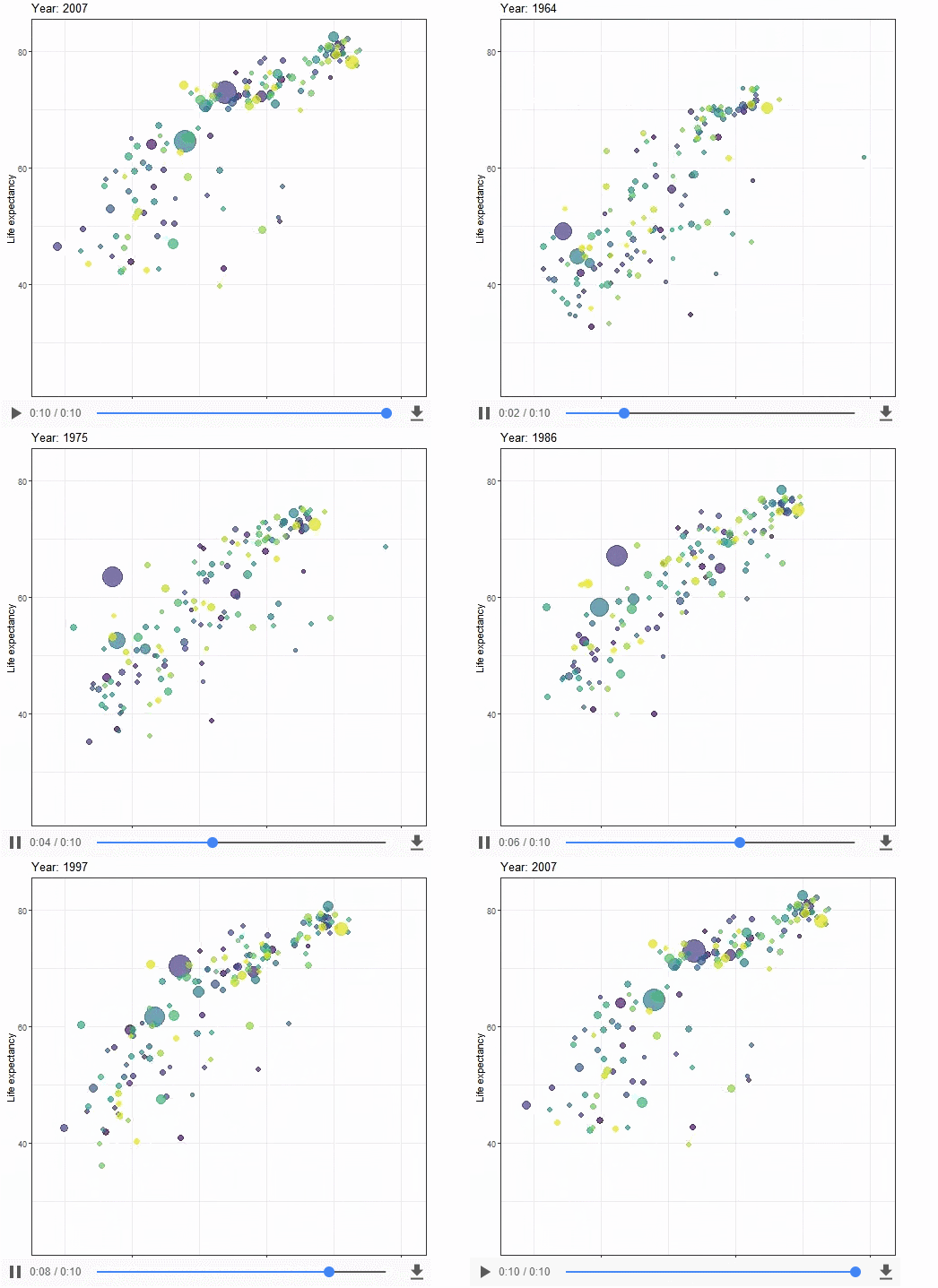
library(ggplot2)
library(gganimate)
theme_set(theme_bw())
library(gapminder)
head(gapminder)
p <- ggplot(
  gapminder, 
  aes(x = gdpPercap, y=lifeExp, size = pop, colour = country)
) +
  geom_point(show.legend = FALSE, alpha = 0.7) +
  scale_color_viridis_d() +
  scale_size(range = c(2, 12)) +
  scale_x_log10() +
  labs(x = "GDP per capital", y = "Life expectancy")
p + transition_time(year) +
  labs(title = "Year: {frame_time}")
1
2
3
4
5
6
7
8
9
10
11
12
13
14
15
16

根据不同大洲创建不同面:

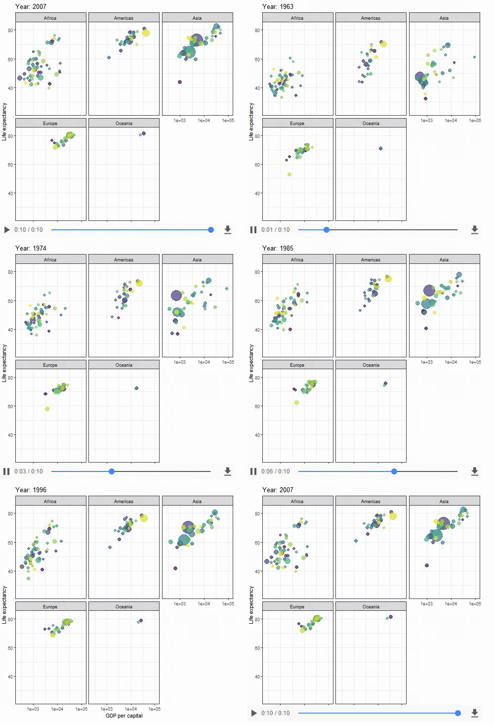
library(ggplot2)
library(gganimate)
theme_set(theme_bw())
library(gapminder)
head(gapminder)
p <- ggplot(
  gapminder, 
  aes(x = gdpPercap, y=lifeExp, size = pop, colour = country)
) +
  geom_point(show.legend = FALSE, alpha = 0.7) +
  scale_color_viridis_d() +
  scale_size(range = c(2, 12)) +
  scale_x_log10() +
  labs(x = "GDP per capital", y = "Life expectancy")
p + facet_wrap(~continent) +
  transition_time(year) +
  labs(title = "Year: {frame_time}")
1
2
3
4
5
6
7
8
9
10
11
12
13
14
15
16
17

让视图跟着每帧数据变

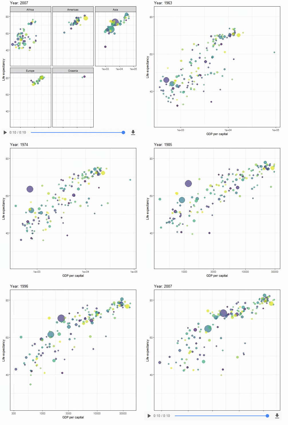
p + transition_time(year) +
  labs(title = "Year: {frame_time}") +
  view_follow(fixed_y = TRUE)
1
2
3

Show preceding frames with gradual falloff
This shadow is meant to draw a small wake after data by showing the latest frames up to the current. You can choose to gradually diminish the size and/or opacity of the shadow. The length of the wake is not given in absolute frames as that would make the animation susceptible to changes in the framerate. Instead it is given as a proportion of the total length of the animation.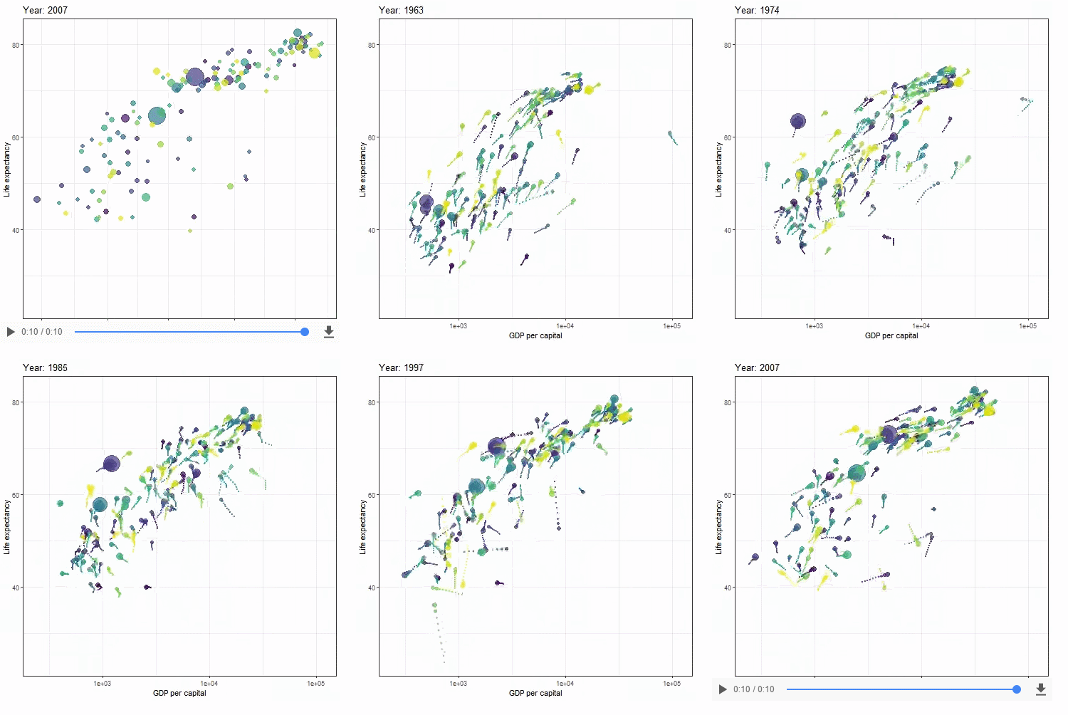

Show the original data as background marks
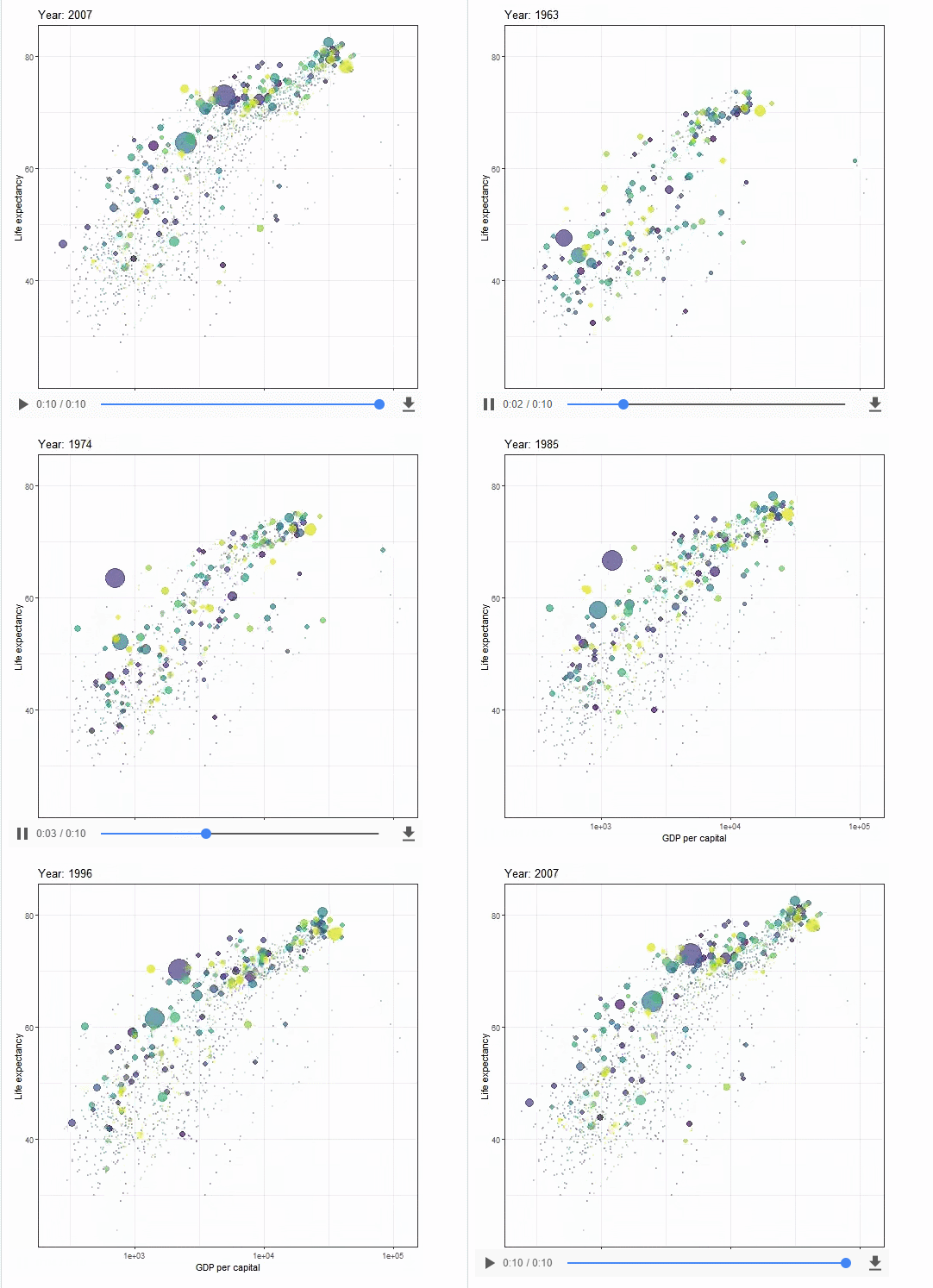
This shadow lets you show the raw data behind the current frame. Both past and/or future raw data can be shown and styled as you want.

p + transition_time(year) +
  labs(title = "Year: {frame_time}") +
  shadow_wake(wake_length = 0.1, alpha = FALSE)
1
2
3

Reveal data along a given dimension
This transition allows you to let data gradually appear, based on a given time dimension.

Static plot

p + transition_time(year) +
  labs(title = "Year: {frame_time}") +
  shadow_mark(alpha = 0.3, size = 0.5)
1
2
3

Let data gradually appear
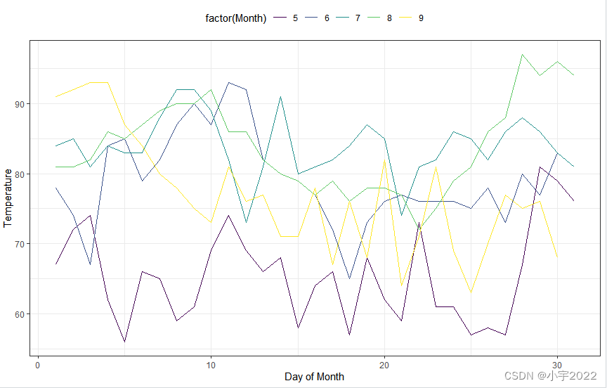
Reveal by day (x-axis)

library(ggplot2)
library(gganimate)
theme_set(theme_bw())
library(gapminder)
p <- ggplot(
  airquality,
  aes(Day, Temp, group = Month, color = factor(Month))
) +
  geom_line() +
  scale_color_viridis_d() +
  labs(x = "Day of Month", y = "Temperature") +
  theme(legend.position = "top")
p
1
2
3
4
5
6
7
8
9
10
11
12
13

Show points:

p + transition_reveal(Day)
1

Points can be kept by giving them a unique group:

p + 
  geom_point() +
  transition_reveal(Day)
1
2
3

Transition between several distinct stages of the data
Create a bar plot of mean temperature:

p + 
  geom_point(aes(group = seq_along(Day))) +
  transition_reveal(Day)
1
2
3

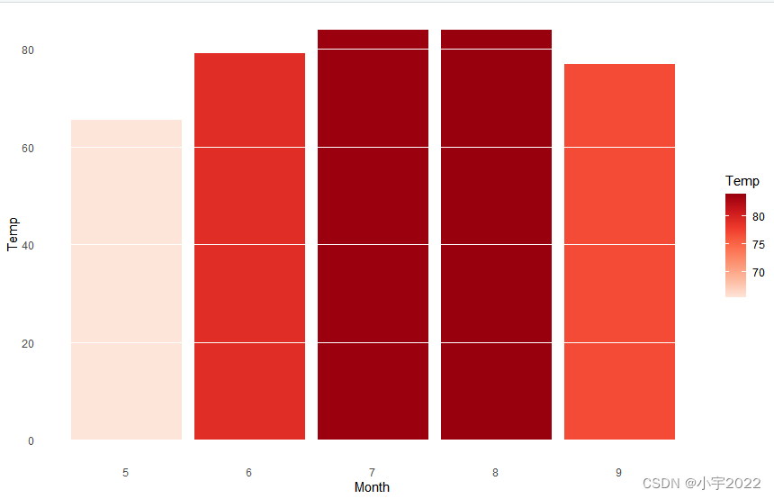
transition_states():

library(dplyr)
mean.temp <- airquality %>%
  group_by(Month) %>%
  summarise(Temp = mean(Temp))
mean.temp
p <- ggplot(mean.temp, aes(Month, Temp, fill = Temp)) +
  geom_col() +
  scale_fill_distiller(palette = "Reds", direction = 1) +
  theme_minimal() +
  theme(
    panel.grid = element_blank(),
    panel.grid.major.y = element_line(color = "white"),
    panel.ontop = TRUE
  )
p
1
2
3
4
5
6
7
8
9
10
11
12
13
14
15

library(dplyr)
mean.temp <- airquality %>%
  group_by(Month) %>%
  summarise(Temp = mean(Temp))
mean.temp
p <- ggplot(mean.temp, aes(Month, Temp, fill = Temp)) +
  geom_col() +
  scale_fill_distiller(palette = "Reds", direction = 1) +
  theme_minimal() +
  theme(
    panel.grid = element_blank(),
    panel.grid.major.y = element_line(color = "white"),
    panel.ontop = TRUE
  )
p + transition_states(Month, wrap = FALSE) +
  shadow_mark()
1
2
3
4
5
6
7
8
9
10
11
12
13
14
15
16

enter_grow() + enter_fade()

p + transition_states(Month, wrap = FALSE) +
  shadow_mark() +
  enter_grow() +
  enter_fade()
1
2
3
4

参考资料：

https://www.datanovia.com/en/blog/gganimate-how-to-create-plots-with-beautiful-animation-in-r/
https://cloud.tencent.com/developer/article/1675209
TED：https://www.ted.com/talks/hans_rosling_the_best_stats_you_ve_ever_seenlanguage=zh-TW