深度学习复盘与论文复现B

1、Knowledge Review

1.1 NLLLoss vs CrossEntropyLoss

NLLoss: 官方网站

import torch

z = torch.Tensor([[0.2, 0.1, -0.1]])
y = torch.LongTensor([0])

criterion = torch.nn.CrossEntropyLoss()

loss = criterion(z, y)
print(loss)

• 在PyTorch中，torch.LongTensor 是一个用于存储长整型（long）数据的张量（tensor）。y = torch.LongTensor([0]) 创建了一个包含单个元素 0 的长整型张量。

import numpy as np

z = np.array([0.2, 0.1, -0.1])
y = np.array([1, 0, 0])

y_pred = np.exp(z) / np.exp(z).sum()
print(y_pred)

loss = (- y * np.log(y_pred)).sum()
print(loss)

CrossEntropyLoss： 官方网站

CrossEntropyLoss <==> LogSoftmax+NLLLoss

• 神经网络的最后一层不需要做激活（经过Softmax层的计算），直接输入到CrossEntropyLoss损失函数中即可。

1.2 MNIST dataset

1.2.1 Repare Dataset

batch_size = 64

transform = transforms.Compose([
    transforms.ToTensor(),  # 将PIL Image 转换为 Tensor
    transforms.Normalize((0.1307,), (0.3081,))  # 均值 和 标准差
])

train_dataset = datasets.MNIST(root='../data/mnist', train=True, download=True, transform=transform)
train_loader = DataLoader(train_dataset, shuffle=True, batch_size=batch_size)

test_dataset = datasets.MNIST(root='../data/mnist', train=False, download=True, transform=transform)
test_loader = DataLoader(test_dataset, shuffle=False, batch_size=batch_size)

Normalize((mean, ), (std, ))：均值 标准差，数据归一化

$$Pixe{l}_{\text{norm}}=\frac{Pixe{l}_{\text{origin}}-\text{mean}}{\text{std}}$$

1.2.2 Design Model

class Net(torch.nn.Module):
    def __init__(self):
        super(Net, self).__init__()
        self.l1 = torch.nn.Linear(784, 512)
        self.l2 = torch.nn.Linear(512, 256)
        self.l3 = torch.nn.Linear(256, 128)
        self.l4 = torch.nn.Linear(128, 64)
        self.l5 = torch.nn.Linear(64, 10)

    def forward(self, x):
        x = x.view(-1, 784)    # 28x28 = 784
        x = F.relu(self.l1(x))
        x = F.relu(self.l2(x))
        x = F.relu(self.l3(x))
        x = F.relu(self.l4(x))
        return self.l5(x)  # 最后一层 不需要激活


model = Net()

C W H == 通道数 宽 高

• 在PyTorch中，view() 方法用于重新调整张量（Tensor）的形状。它 将一个张量重塑（reshape）为具有指定形状的新张量。这个方法在神经网络中尤其有用，当需要将张量从一种形状转换为另一种形状以适应模型的某个层时。

1.2.3 Construct Loss and Optimizer

criterion = torch.nn.CrossEntropyLoss()
optimizer = optim.SGD(model.parameters(), lr=0.01, momentum=0.5) 

1.2.4 Train and Test

def train(epoch):
    running_loss = 0.0
    for batch_idx, data in enumerate(train_loader, 0):
        inputs, target = data
        optimizer.zero_grad()  # 清零

        # forward + backward + update
        outputs = model(inputs)
        loss = criterion(outputs, target)
        loss.backward()
        optimizer.step()

        running_loss += loss.item()
        if batch_idx % 300 == 299:
            print('[%d, %5d] loss: %.3f' % (epoch + 1, batch_idx + 1, running_loss / 300))
            running_loss = 0.0


def test():
    correct = 0
    total = 0
    with torch.no_grad():  # 不需要计算梯度
        for data in test_loader:
            images, labels = data
            outputs = model(images)
            _, predicted = torch.max(outputs, dim=1)
            total += labels.size(0)
            correct += (predicted == labels).sum().item()
    print('Accuracy on test set: %d %%' % (100 * correct / total))


if __name__ == '__main__':
    for epoch in range(10):
        train(epoch)
        test()

1.2.5 Training results

Pytorch-Lightning MNIST 🚀🔥

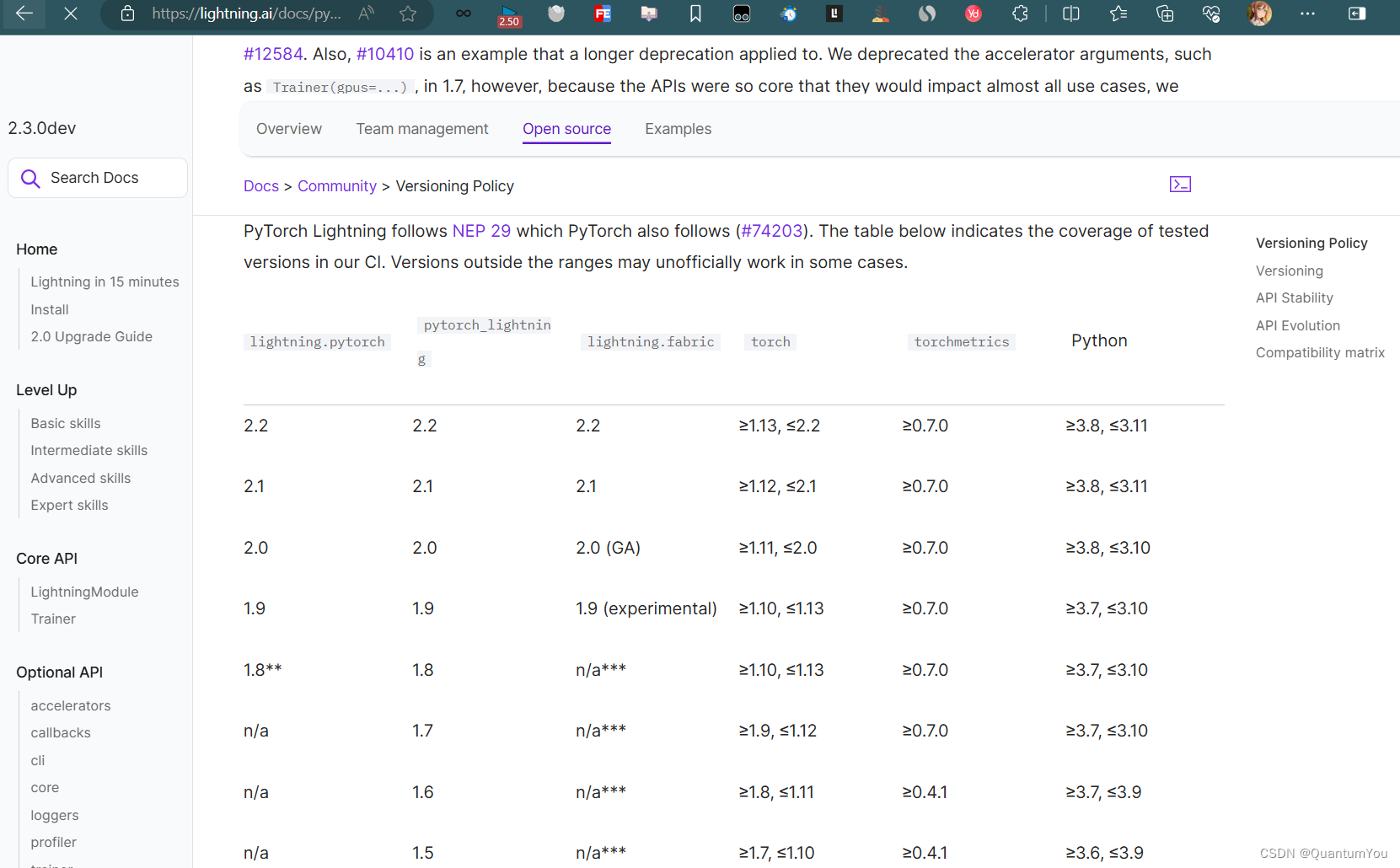
https://lightning.ai/docs/pytorch/latest/versioning.html#pytorch-support

推荐文章: https://evernorif.github.io/2024/01/19/Pytorch-Lightning%E5%BF%AB%E9%80%9F%E5%85%A5%E9%97%A8/#quick-start

• 通过使用 Pytorch-Lightning 正式开始训练
  

1.3 Basic Convolutional Neural Networks

1.3.1 Introduction

• 1 × 28 × 28 < = = > C × W × H

• Convolution 卷积：保留图像的空间结构信息

• Subsampling 下采样（主要是 Max Pooling）：通道数不变，宽高改变，为了减少图像数据量，进一步降低运算的需求

• Fully Connected 全连接：将张量展开为一维向量，再进行分类

• 我们将 Convolution 及 Subsampling 等称为特征提取（Feature Extraction），最后的 Fully Connected 称为分类（Classification）。

1.3.2 Convolution

栅格图像（Raster Graphics）和矢量图像（Vector Graphics）
区别：

1. 存储方式：

   • 栅格图像是以点阵形式存储的，它的基本元素是像素（像元），图像信息是以像素灰度的矩阵形式记录的。
   • 矢量图像是以矢量形式存储的，它的基本元素是图形要素，图形要素的几何形状是以坐标方式按点、线、面结构记录的。

2. 显示方式：

   • 栅格图像的显示是逐行、逐列、逐像元地显示，与内容无关。
   • 矢量图形的显示是逐个图形要素按顺序地显示，显示位置的先后没有规律。

3. 缩放效果：

   • 栅格图像放大到一定的倍数时，图像信息会发生失真，特别是图像目标的边界会发生阶梯效应。
   • 矢量图形的放大和缩小，其图形要素、目标不会发生失真。

4. 存储空间：

   • 表示效果相同时，栅格图像表示比矢量图形表示所占用的存储空间大得多。

5. 颜色与细节：

   • 栅格图像可以支持广泛的颜色范围并描绘细致的阶调，非常适合显示连续色调图像，如照片或有阴影的绘画。
   • 矢量图形在色彩层次丰富的逼真图像效果上表现较为困难。

1.3.3 Channel

• Single Input Channel：
  

注意进行的操作是数乘

• 3 Input Channels：

每个通道配一个核

• N Input Channels：
  
• N Input Channels and M Output Channels

卷积核通道数=输入通道数，卷积核个数=输出通道数

import torch

in_channels, out_channels = 5, 10
width, height = 100, 100
kernel_size = 3
batch_size = 1

input = torch.randn(batch_size, in_channels, width, height)
conv_layer = torch.nn.Conv2d(in_channels, out_channels, kernel_size=kernel_size)
output = conv_layer(input)

print(input.shape)
print(conv_layer.weight.shape)  # m n w h
print(output.shape)

1.3.4 Padding

Ouput=(Input+2∗padding−kernel)/stride+1

import torch

input = [3, 4, 6, 5, 7,
         2, 4, 6, 8, 2,
         1, 6, 7, 8, 4,
         9, 7, 4, 6, 2,
         3, 7, 5, 4, 1]

input = torch.Tensor(input).view(1, 1, 5, 5)  # B C W H

conv_layer = torch.nn.Conv2d(in_channels=1, out_channels=1, kernel_size=3, padding=1, bias=False)  # O I W H
kernel = torch.Tensor([1, 2, 3, 4, 5, 6, 7, 8, 9]).view(1, 1, 3, 3)
conv_layer.weight.data = kernel.data

output = conv_layer(input)

print(output)

• Stride：参数 stride 意为步长，假设stride = 2 时，kernel在向右或向下移动时，一次性移动两格，可以有效的降低图像的宽度和高度。 🚀🚀

1.3.5 Max Pooling

• Max Pooling：最大池化，默认 stride = 2 ，若 kernel = 2 ，即在该表格中找出最大值：
  

import torch

input = [3, 4, 6, 5,
         2, 4, 6, 8,
         1, 6, 7, 8,
         9, 7, 4, 6]

input = torch.Tensor(input).view(1, 1, 4, 4)
maxpooling_layer = torch.nn.MaxPool2d(kernel_size=2)
output = maxpooling_layer(input)

print(output)

1.4 Implementation of CNN

• 28x28 --> 24x24 的原因： (28+2x0-5)/1+1 = 24
• 24x24 --> 12x12 的原因 (24+2x0-2)/2+1= 12
• 12x12 --> 8x8 的原因： （12+2x0-5)/1+1=8
• 8x8 --> 4x4 的原因： （8+2x0-2)/2+1 = 4

Ouput=(Input+2∗padding−kernel)/stride+1

1.4.1 Fully Connected Neural Network

class Net(torch.nn.Module):
    def __init__(self):
        super(Net, self).__init__()
        self.conv1 = torch.nn.Conv2d(1, 10, kernel_size=5)
        self.conv2 = torch.nn.Conv2d(10, 20, kernel_size=5)
        self.pooling = torch.nn.MaxPool2d(2)
        self.fc = torch.nn.Linear(320, 10)

    def forward(self, x):
        # Flatten data from (n, 1, 28, 28) to (n, 784)
        batch_size = x.size(0)
        x = F.relu(self.pooling(self.conv1(x)))
        x = F.relu(self.pooling(self.conv2(x)))
        x = x.view(batch_size, -1)  # flatten
        x = self.fc(x)
        return x


model = Net()

1.4.2 CUDA PyTorch GPU

• Move Model to GPU ：在调用模型后添加以下代码

device = torch.device("cuda:0" if torch.cuda.is_available() else "cpu")
model.to(device)

• Move Tensors to GPU ：训练和测试函数添加以下代码

inputs, target = inputs.to(device), target.to(device)

1.4.3 Training results

1.5 Advanced Convolutional Neural Networks

1.5.1 GoogLeNet ReView

• 若以上图来编写神经网络，则会有许多重复，为减少代码冗余，可以尽量多使用函数/类。

1.5.2 Inception Module

GoogLeNet在一个块中将几种卷积核（1×1、3×3、5×5、…）都使用，然后将其结果罗列到一起，将来通过训练自动找到一种最优的组合。

• Concatenate：将张量拼接到一块

• Average Pooling 均值池化：保证输入输出宽高一致（可借助padding和stride）

1x1的卷积核主要作用就是降维

1.5.3 Implementation of Inception Module

# 第一列
self.branch_pool = nn.Conv2d(in_channels, 24, kernel_size=1)

branch_pool = F.avg_pool2d(x, kernel_size=3, stride=1, padding=1)
branch_pool = self.branch_pool(branch_pool)

# 第二列
self.branch1x1 = nn.Conv2d(in_channels, 16, kernel_size=1)

branch1x1 = self.branch1x1(x)

# 第三列
self.branch5x5_1 = nn.Conv2d(in_channels,16, kernel_size=1)
self.branch5x5_2 = nn.Conv2d(16, 24, kernel_size=5, padding=2)

branch5x5 = self.branch5x5_1(x)
branch5x5 = self.branch5x5_2(branch5x5)

# 第四列
self.branch3x3_1 = nn.Conv2d(in_channels, 16, kernel_size=1)
self.branch3x3_2 = nn.Conv2d(16, 24, kernel_size=3, padding=1)
self.branch3x3_3 = nn.Conv2d(24, 24, kernel_size=3, padding=1)

branch3x3 = self.branch3x3_1(x)
branch3x3 = self.branch3x3_2(branch3x3)
branch3x3 = self.branch3x3_3(branch3x3)

1.5.4 Residual Net ReView

Paper: He K, Zhang X, Ren S, et al. Deep Residual Learning for Image Recognition[C]// IEEE Conference on Computer Vision and Pattern Recognition. IEEE Computer Society, 2016:770-778

1. 残差学习的思想：

   • 在传统的卷积神经网络中，每一层的输出都是由前一层的输入经过卷积、激活函数等操作得到的。
   • 而在ResNet中，每一层的输出不仅包括前一层的输出，还包括前一层的输入。这样做的目的是为了让网络可以学习到残差，即前一层的输入与输出之间的差异，从而更好地拟合数据。

2. 残差模块（Residual Block）：

   • ResNet中的每个基本块（Basic Block）都由两个卷积层和一个跳跃连接（Shortcut Connection）组成。
   • 跳跃连接将前一层的输入直接加到当前层的输出上，从而形成了一个残差块。这样做的好处是，即使当前层的输出与前一层的输入相差很大，跳跃连接也可以让信息直接传递到后面的层，避免了信息的丢失。

3. 网络结构：

   • ResNet由多个基本块组成，其中每个基本块的输出都是由前一个基本块的输出和前一层的输入相加得到的。
   • 这种结构允许信息在不同的层之间自由地流动，从而避免了梯度消失和梯度爆炸问题。

class Net(nn.Module):
    def __init__(self):
        super(Net, self).__init__()
        self.conv1 = nn.Conv2d(1, 16, kernel_size=5)
        self.conv2 = nn.Conv2d(16, 32, kernel_size=5)
        self.mp = nn.MaxPool2d(2)
        self.rblock1 = ResidualBlock(16)
        self.rblock2 = ResidualBlock(32)
        self.fc = nn.Linear(512, 10)

    def forward(self, x):
        in_size = x.size(0)
        x = self.mp(F.relu(self.conv1(x)))
        x = self.rblock1(x)
        x = self.mp(F.relu(self.conv2(x)))
        x = self.rblock2(x)
        x = x.view(in_size, -1)
        x = self.fc(x)
        return x

1.5.5 Residual Block

class ResidualBlock(nn.Module):
    def __init__(self, channels):
        super(ResidualBlock, self).__init__()
        self.channels = channels
        self.conv1 = nn.Conv2d(channels, channels, kernel_size=3, padding=1)
        self.conv2 = nn.Conv2d(channels, channels, kernel_size=3, padding=1)

    def forward(self, x):
        y = F.relu(self.conv1(x))
        y = self.conv2(y)
        return F.relu(x + y)

注意仔细看 颜色对应代码图片

1.5.6 Train and Test

1.5.7 Reading Paper

• Paper: Paper He K, Zhang X, Ren S, et al. Identity Mappings in Deep Residual Networks[C]

• Paper: Huang G, Liu Z, Laurens V D M, et al. Densely Connected Convolutional Networks[J]. 2016:2261-2269.

2、Recurrent Neural Network

2.1 RNN Cell in PyTorch

• 用于处理一些具有前后关系的序列问题。

import torch

batch_size=1
seq_len=3
input_size=4
hidden_size=2
 
Cell=torch.nn.RNNCell(input_size=input_size,hidden_size=hidden_size)#初始化，构建RNNCell
 
dataset=torch.randn(seq_len,batch_size,input_size)#设置dataset的维度
print(dataset)
 
hidden=torch.zeros(batch_size,hidden_size)#隐层的维度：batch_size*hidden_size，先把h0置为0向量
 
for idx,input in enumerate(dataset):
    print('='*10,idx,'='*10)
    print('Input size:',input.shape)
    
    hidden=Cell(input,hidden)
    print('Outputs size:',hidden.shape)
    print(hidden)

2.2 Application of RNN

• seqSize就是指天气的第一天，第二天，第三天一共3天
• seq_len指的是一天中的气压，温度，湿度等信息

import torch
batch_size=1
seq_len=3
input_size=4
hidden_size=2
num_layers=1
cell=torch.nn.RNN(input_size=input_size,hidden_size=hidden_size,num_layers=num_layers)
#构造RNN时指明输入维度，隐层维度以及RNN的层数
inputs=torch.randn(seq_len,batch_size,input_size)
hidden=torch.zeros(num_layers,batch_size,hidden_size)
out,hidden=cell(inputs,hidden)
print('Output size:',out.shape)
print('Output:',out)
print('Hidden size:',hidden.shape)
print('Hidden',hidden)

2.3 Using RNNCell

#使用RNN
import torch
 
input_size=4
hidden_size=4
num_layers=1
batch_size=1
seq_len=5
# 准备数据
idx2char=['e','h','l','o'] # 0 1 2 3
x_data=[1,0,2,2,3] # hello
y_data=[3,1,2,3,2] # ohlol
 
# e h l o
one_hot_lookup=[[1,0,0,0],
                [0,1,0,0],
                [0,0,1,0],
                [0,0,0,1]] #分别对应0,1,2,3项
x_one_hot=[one_hot_lookup[x] for x in x_data] # 组成序列张量
print('x_one_hot:',x_one_hot)
 
# 构造输入序列和标签
inputs=torch.Tensor(x_one_hot).view(seq_len,batch_size,input_size)
print(inputs)
labels=torch.LongTensor(y_data)  #labels维度是: (seqLen * batch_size ，1)
print(labels)
 
# design model
class Model(torch.nn.Module):
    def __init__(self,input_size,hidden_size,batch_size,num_layers=1):
        super(Model, self).__init__()
        self.num_layers=num_layers
        self.batch_size=batch_size
        self.input_size=input_size
        self.hidden_size=hidden_size
        self.rnn=torch.nn.RNN(input_size=self.input_size,
                              hidden_size=self.hidden_size,
                              num_layers=self.num_layers)
 
    def forward(self,input):
        hidden=torch.zeros(self.num_layers,self.batch_size,self.hidden_size)
        out, _=self.rnn(input,hidden)
        # 为了能和labels做交叉熵，需要reshape一下:(seqlen*batchsize, hidden_size),即二维向量，变成一个矩阵
        return out.view(-1,self.hidden_size)
 
net=Model(input_size,hidden_size,batch_size,num_layers)
 
# loss and optimizer
criterion=torch.nn.CrossEntropyLoss()
optimizer=torch.optim.Adam(net.parameters(), lr=0.05)
 
# train cycle
for epoch in range(20):
    optimizer.zero_grad()
    #inputs维度是: (seqLen, batch_size, input_size) labels维度是: (seqLen * batch_size * 1)
    #outputs维度是: (seqLen, batch_size, hidden_size)
    outputs=net(inputs)
    loss=criterion(outputs,labels)
    loss.backward()
    optimizer.step()
 
    _, idx=outputs.max(dim=1)
    idx=idx.data.numpy()
    print('Predicted: ',''.join([idx2char[x] for x in idx]),end='')
    print(',Epoch [%d/20] loss=%.3f' % (epoch+1, loss.item()))

2.4 One-hot vs Embedding

跳转链接

 
 #Embedding编码方式
import torch
 
input_size = 4
num_class = 4
hidden_size = 8
embedding_size = 10
batch_size = 1
num_layers = 2
seq_len = 5
 
idx2char_1 = ['e', 'h', 'l', 'o']
idx2char_2 = ['h', 'l', 'o']
 
x_data = [[1, 0, 2, 2, 3]]
y_data = [3, 1, 2, 2, 3]
 
# inputs 维度为（batchsize，seqLen）
inputs = torch.LongTensor(x_data)
# labels 维度为（batchsize*seqLen）
labels = torch.LongTensor(y_data)
 
 
class Model(torch.nn.Module):
    def __init__(self):
        super(Model, self).__init__()
        #告诉input大小和 embedding大小 ，构成input_size * embedding_size 的矩阵
        self.emb = torch.nn.Embedding(input_size, embedding_size)
 
        self.rnn = torch.nn.RNN(input_size=embedding_size,
                                hidden_size=hidden_size,
                                num_layers=num_layers,
                                batch_first=True)
        # batch_first=True，input of RNN:(batchsize,seqlen,embeddingsize) output of RNN:(batchsize,seqlen,hiddensize)
        self.fc = torch.nn.Linear(hidden_size, num_class) #从hiddensize 到 类别数量的 变换
 
    def forward(self, x):
        hidden = torch.zeros(num_layers, x.size(0), hidden_size)
        x = self.emb(x)  # 进行embedding处理，把输入的长整型张量转变成嵌入层的稠密型张量
        x, _ = self.rnn(x, hidden)
        x = self.fc(x)
        return x.view(-1, num_class) #为了使用交叉熵，变成一个矩阵（batchsize * seqlen,numclass）
 
 
net = Model()
 
criterion = torch.nn.CrossEntropyLoss()
optimizer = torch.optim.Adam(net.parameters(), lr=0.05)
 
for epoch in range(15):
    optimizer.zero_grad()
    outputs = net(inputs)
 
    loss = criterion(outputs, labels)
    loss.backward()
    optimizer.step()
 
    _, idx = outputs.max(dim=1)
    idx = idx.data.numpy()
    print('Predicted string: ', ''.join([idx2char_1[x] for x in idx]), end='')
    print(", Epoch [%d/15] loss = %.3f" % (epoch + 1, loss.item())

2.5 Preliminary Introduction to LSTM

跳转链接

总结：一般LSTM 比RNN性能好，但运算性能时间复杂度比较高，所以引出折中的GRU介绍

2.6 GRU Introduction

跳转地址

• 嵌入层（Embedding Layer）是深度学习模型中常见的一种层，其主要作用是将高维稀疏特征转化为低维稠密向量。

1. 嵌入层的作用：

• 降维与升维：嵌入层能够对输入数据进行降维或升维处理。在自然语言处理中，常常使用独热编码（One-Hot Encoding）来表示词汇，但这种表示方法会导致向量维度过高且稀疏。嵌入层可以将这些高维稀疏向量映射到低维稠密空间，同时保留词汇间的语义关系。此外，在某些情况下，嵌入层也可用于升维，以更细致地刻画数据特征。
• 特征表示：通过嵌入层，每个输入特征（如单词、用户ID等）都被映射到一个固定长度的向量。这种向量表示能够捕捉特征之间的相似性和关联性，有助于模型更好地理解和处理输入数据。
• 优化模型性能：嵌入层的参数在训练过程中会不断优化，使得模型能够学习到更好的特征表示。这有助于提高模型的性能和准确率。

2. 嵌入层的工作原理：

• 索引查找：在输入序列中，每个离散特征都表示为一个整数索引。嵌入层首先根据这些索引找到对应的行向量。
• 向量映射：然后，嵌入层将找到的行向量进行线性映射，将它们映射到指定的输出维度。这个映射通常通过矩阵乘法实现。

3、Kaggle Titanic achieve

跳转地址