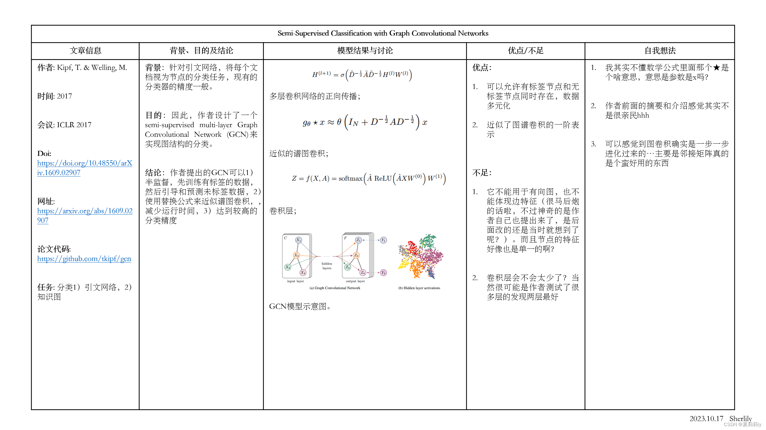
[论文精读]Semi-Supervised Classification with Graph Convolutional Networks

[论文精读]Semi-Supervised Classification with Graph Convolutional Networks

论文原文：[1609.02907] Semi-Supervised Classification with Graph Convolutional Networks (arxiv.org)

论文代码：GitHub - tkipf/gcn: Implementation of Graph Convolutional Networks in TensorFlow

英文是纯手打的！论文原文的summarizing and paraphrasing。可能会出现难以避免的拼写错误和语法错误，若有发现欢迎评论指正！文章偏向于笔记，谨慎食用！

目录

1. 省流版

1.1. 心得

1.2. 论文框架图

2. 论文逐段阅读

2.1. Abstract

2.2. Introduction

2.3. Fast approximate convolutions on graphs

2.3.1. Spectral graph convolutions

2.3.2. Layer-wise linear model

2.4. Semi-supervised node classification

2.4.1. Example

2.4.2. Implementation

2.5. Related work

2.5.1. Graph-based semi-supervised learning

2.5.2. Neural networks on graphs

2.6. Experiments

2.6.1. Datasets

2.6.2. Experimental set-up

2.6.3. Baselines

2.7. Results

2.7.1. Semi-supervised node classifiication

2.7.2. Evaluation of propagation model

2.7.3. Training time per epoch

2.8. Discussion

2.8.1. Semi-supervised model

2.8.2. Limitations and future work

2.9. Conclusion

3. 知识补充

3.1. Skip-gram

3.2. Bag of words

3.3. Spectral graph convolutions

4. Reference List

1. 省流版

1.1. 心得

（1）怎么开头我就不知道在说什么啊这个论文感觉表述不是很清晰？

（2）数学部分推理很清晰

（3）要是模型展示更清晰就好了

1.2. 论文框架图

2. 论文逐段阅读

2.1. Abstract

①Their convolution is based on localized first-order approximation

②They encode node features and local graph structure in hidden layers

2.2. Introduction

①The authors think adopting Laplacian regularization in the loss function helps to label:

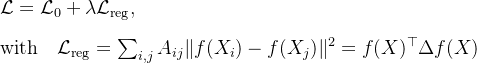
$\mathcal{L}=\mathcal{L}_0+\lambda\mathcal{L}_{\text{reg}},\quad\\\\\text{with}\quad\mathcal{L}_{\text{reg}}=\sum_{i,j}A_{ij}\|f(X_i)-f(X_j)\|^2=f(X)^\top\Delta f(X)$

where $\mathcal{L}_0$ represents supervised loss with labeled data,

$f\left ( \right )$ is a differentiable function,

$\lambda$ denotes weight,

denotes matrix with combination of node feature vectors,

$\triangle =D-A$ represents the unnormalized graph Laplacian,

is adjacency matrix,

is degree matrix.

②The model trains labeled nodes and is able to learn labeled and unlabeled nodes

③GCN achieves higher accuracy and efficiency than others

2.3. Fast approximate convolutions on graphs

①GCN (undirected graph):

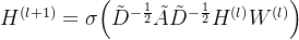
$H^{(l+1)}=\sigma\Big(\tilde{D}^{-\frac{1}{2}}\tilde{A}\tilde{D}^{-\frac{1}{2}}H^{(l)}W^{(l)}\Big)$

where 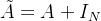$\tilde{A}$ denotes self-connection adjacency matrix, which means $\tilde{A}=A+I_{N}$ ,

$I_{N}$ denotes identity matrix,

$\tilde{D}$ denotes self-connection degree matrix,

$W^{(l)}$ represents the trainable weight matrix in -th layer,

$H^{(l)}$ denotes the activation matrix in -th layer,

$\sigma \left ( \right )$ represents activation function

2.3.1. Spectral graph convolutions

①Spectral convolutions on graphs:

$g_{\theta }\star x=Ug_{\theta }U^{T}x$

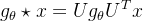
where the filter $g_{\theta }=diag\left ( \theta \right )$ ,

comes from normalized graph Laplacian $L=I_{N}-D^{-\frac12}AD^{-\frac12}=U\Lambda U^{T}$ and is the matrix of 's eigenvectors,

$\Lambda$ denotes a diagonal matrix with eigenvalues.

②However, it is too time-consuming to compute matrix especially for large graph. Ergo, approximating it in -th order by Chebyshev polynomials:

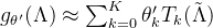
$g_{\theta^{\prime}}(\Lambda)\approx\sum_{k=0}^K\theta_k^{\prime}T_k(\tilde{\Lambda})$

where $\tilde{\Lambda}=\frac{2}{\lambda_{\max}}\Lambda-I_{N}$ ,

${\theta }'$ denotes Chebyshev coefficients vector,

recursive Chebyshev polynomials are $T_{k}\left ( x \right )=2xT_{k-1}(x)-T_{k-2}(x)$ with baseline $T_{0}(x)=1$ and $T_{1}(x)=x$

③Then get new function:

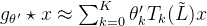
$g_{\theta'}\star x\approx\sum_{k=0}^{K}\theta'_kT_k(\tilde{L})x$

where $\tilde{L}=\frac{2}{\lambda_{\max}}L-I_{N}$ , $(U\Lambda U^\top)^k=U\Lambda^kU^\top$ .

④Through this approximation method, time complexity reduced from $O\left ( n^{2} \right )$ to $O\left ( E \right )$

2.3.2. Layer-wise linear model

①Then, the authors stack the function above to build multiple conv layers and set , $\lambda _{max}\approx 2$

②They simplified 2.3.1. ③ to:

$g_{\theta'}\star x\approx\theta'_0x+\theta'_1\left(L-I_N\right)x=\theta'_0x-\theta'_1D^{-\frac{1}{2}}AD^{-\frac{1}{2}}x$

where $\theta'_0$ and $\theta'_1$ are free parameters

③Nevertheless, more parameters bring more overfitting problem. It leads the authors change the expression to:

$g_\theta\star x\approx\theta\left(I_N+D^{-\frac{1}{2}}AD^{-\frac{1}{2}}\right)x$

where they define $\theta=\theta_0^{\prime}=-\theta_1^{\prime}$ ,

eigenvalues are in $\left [ 0,2 \right ]$ .

But keep using it may cause exploding/vanishing gradients or numerical instabilities.

④Then they adjust $I_{N}+D^{-\frac{1}{2}}AD^{-\frac{1}{2}}\rightarrow\tilde{D}^{-\frac{1}{2}}\tilde{A}\tilde{D}^{-\frac{1}{2}}$

⑤The convolved signal matrix $\begin{aligned}Z&\in\mathbb{R}^{N\times F}\end{aligned}$ :

$Z=\tilde{D}^{-\frac12}\tilde{A}\tilde{D}^{-\frac12}X\Theta$

where  denotes input channels, namely feature dimensionality of each node,

denotes the number of filters or feature maps,

$\Theta\in\mathbb{R}^{C\times F}$ represents matrix of filter parameters

2.4. Semi-supervised node classification

The whole model shows:

2.4.1. Example

①They take 2 layers model

②Forward propagation:

$Z=f(X,A)=\text{softmax}\Big(\hat{A}\, \text{ReLU}\Big(\hat{A}XW^{(0)}\Big)W^{(1)}\Big)$

where $W^{(0)}\in\mathbb{R}^{C\times H}$ is a weight matrix with  feature maps, it crosses input layer to hidden layer,

$W^{(1)}\in\mathbb{R}^{H\times F}$ is a weight matrix crossing hidden layer to output layer,

ReLU is for every row

③Cross entropy:

$\mathcal{L}=-\sum_{l\in\mathcal{Y}_L}\sum_{f=1}^FY_{lf}\ln Z_{lf}$

where $\mathcal{Y}_{L}$ is the set of node indices of which nodes with labels

④They adopt mini-batch stochastic gradient descent

2.4.2. Implementation

①Framework: TensorFlow

②Method: sparse-dense matrix multiplications

③Computational complexity: $O\left ( \left | E \right |CHF \right )$

2.5. Related work

2.5.1. Graph-based semi-supervised learning

（1）Previous graph representations:

①Explicit graph Laplacian regularization: such as deep semi-supervised embedding, manifold regularization, label propagation

②Graph-embedding

（2）Recent works:

①DeepWalk

②LINE

③node2vec

2.5.2. Neural networks on graphs

①Briefly introduced other works

②Their approach is based on spectral graph convolutional neural networks

2.6. Experiments

They tested their model in:

①Semi-supervised document classification in citation networks

②Semi-supervised entity classification in a bipartite graph extracted from a knowledge graph

③Evaluation of various graph propagation models

④Run-time analysis on random graphs

bipartite  adj.两部分组成的;有两个部分的

2.6.1. Datasets

①Datasets table:

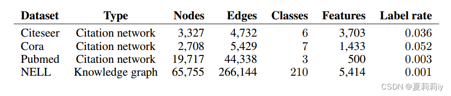
where documents represented by nodes, citation links represented by edges;

also, $Label\, rate=\frac{training\, \, labeled\, \, nodes}{total\, \, nodes}$ ;

NELL is a bipartite graph dataset including 55,864 relation nodes and 9,891 entity nodes

②Citation networks: sparse bag-of-words feature vectors and list of citation links for and between documents are contained. Besides, undirected edges are citation links and 20 labels for one class only

   ③NELL: edges are labeled, directed connections. Additionally, one-hot representation is adopted in each node

④Random graphs: randomly genetate graph with N nodes and 2N edges

2.6.2. Experimental set-up

①Labeled sample test set: 1,000

②They usually adopt 2 layers, but further test extra 10 layers in appendix b

③Epoch: under 200

④Optimizer: Adam

⑤Stop training when there is no decreasing of loss for 10 consecutive epochs

⑥Hidden layer includes 32 units

⑦Omit dropout and regularization

2.6.3. Baselines

①They train local classifier with labeled data and then train unlabeled with a random node ordering for 10 iterations

②L2 regularization parameter and aggregation operator selected by performance of validation set

2.7. Results

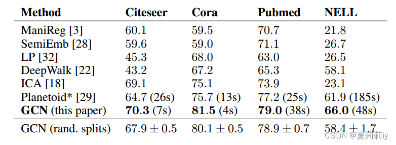
2.7.1. Semi-supervised node classifiication

（1）Comparison of accuracy table with mean accuracy of 100 times in random ordering:

（2）Parameters for Citeseer, Cora and Pubmed

①Dropout rate: 0.5

②L2 regularization: 5e-4

③Hidden units number: 16

（3）Parameters for NELL

①Dropout rate: 0.1

②L2 regularization: 1e-5

③Hidden units number: 64

2.7.2. Evaluation of propagation model

They compared variants of their propagation model on citation network datasets, where GCN is the bold one:

2.7.3. Training time per epoch

Mean training time per epoch of 100 epochs. Each epoch contains forward propagation, cross entropy computing, backward propagation:

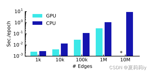
where * denotes memory explosion

2.8. Discussion

2.8.1. Semi-supervised model

①The authors attribute low efficiency of graph-Laplacian regularization to only encoding similar nodes

②In addition, they think skip-gram is hard to optimize

③Then, they reckon renormalized propagation is better than na¨ıve 1 st-order model and higher-order graph convolutional models with Chebyshev polynomials

2.8.2. Limitations and future work

①Lack of memory. Slightly alleviated by mini-batch stochastic gradient descent

②The model does not support directed edge or edge features. （后面说的那句话不是很能理解，翻译成中文是“通过将原始有向图表示为具有原始图中表示边缘的附加节点的无向二部图，可以同时处理有向边和边缘特征”。难道说原本是一个普通的图，把每条边都变成一个节点放在另一边，然后和原先的节点合起来变成二部图？但是很奇怪啊）

③Weight of self-connection might vary in different graphs:

$\tilde{A}=A+\lambda I_{N}$

2.9. Conclusion

They proposed a novel and efficient semi-supervised graph convolutional network

3. 知识补充

3.1. Skip-gram

相关链接：理解 Word2Vec 之 Skip-Gram 模型 - 知乎 (zhihu.com)

3.2. Bag of words

相关链接：使用 Python 的 NLP 中的单词袋简介 |什么是 BoW？ (mygreatlearning.com)

3.3. Spectral graph convolutions

相关链接：谱图卷积 - 知乎 (zhihu.com)

4. Reference List

Kipf, T. & Welling, M. (2017) 'Semi-Supervised Classification with Graph Convolutional Networks', ICLR 2017, doi: https://doi.org/10.48550/arXiv.1609.02907
相关阅读:
SSM框架之MyBatis入门（Maven工程实现全查功能,快速入门，适合小白）
收一个快手协议下单算法
 JNI学习5.jstring的处理
 QT连接数据库
 聚观早报 | 美团打车接入腾讯出行；腾讯音乐将在港交所上市
 【Autosar 存储栈Memery Stack 4.Tc397的Flash编程】
CS信息系统建设和服务能力资质办理指南
 java面向对象----封装 && 构造器
 3.51 什么是平坦式原理图？什么是层次式电路设计？它的优点有哪些？
私域运营如何提高收益？
原文地址：https://blog.csdn.net/Sherlily/article/details/133867185

1. 省流版

1.1. 心得

1.2. 论文框架图

2. 论文逐段阅读

2.1. Abstract

2.2. Introduction

2.3. Fast approximate convolutions on graphs

2.3.1. Spectral graph convolutions

2.3.2. Layer-wise linear model

2.4. Semi-supervised node classification

2.4.1. Example

2.4.2. Implementation

2.5. Related work

2.5.1. Graph-based semi-supervised learning

2.5.2. Neural networks on graphs

2.6. Experiments

2.6.1. Datasets

2.6.2. Experimental set-up

2.6.3. Baselines

2.7. Results

2.7.1. Semi-supervised node classifiication

2.7.2. Evaluation of propagation model

2.7.3. Training time per epoch

2.8. Discussion

2.8.1. Semi-supervised model

2.8.2. Limitations and future work

2.9. Conclusion

3. 知识补充

3.1. Skip-gram

3.2. Bag of words

3.3. Spectral graph convolutions

4. Reference List