《PyTorch深度学习实践》第三讲 梯度下降算法

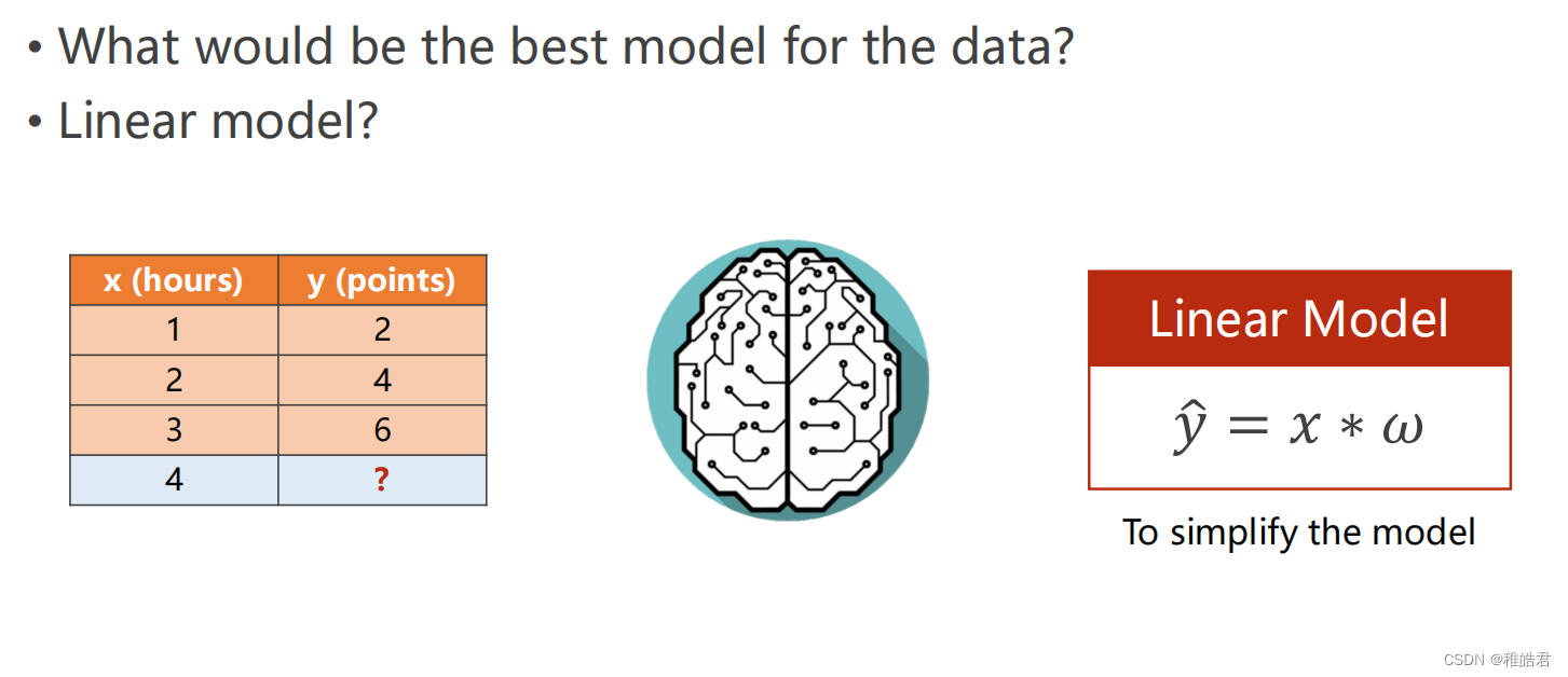
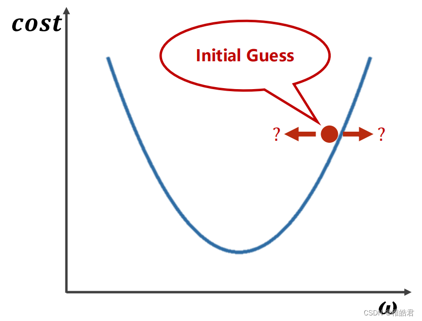
问题描述

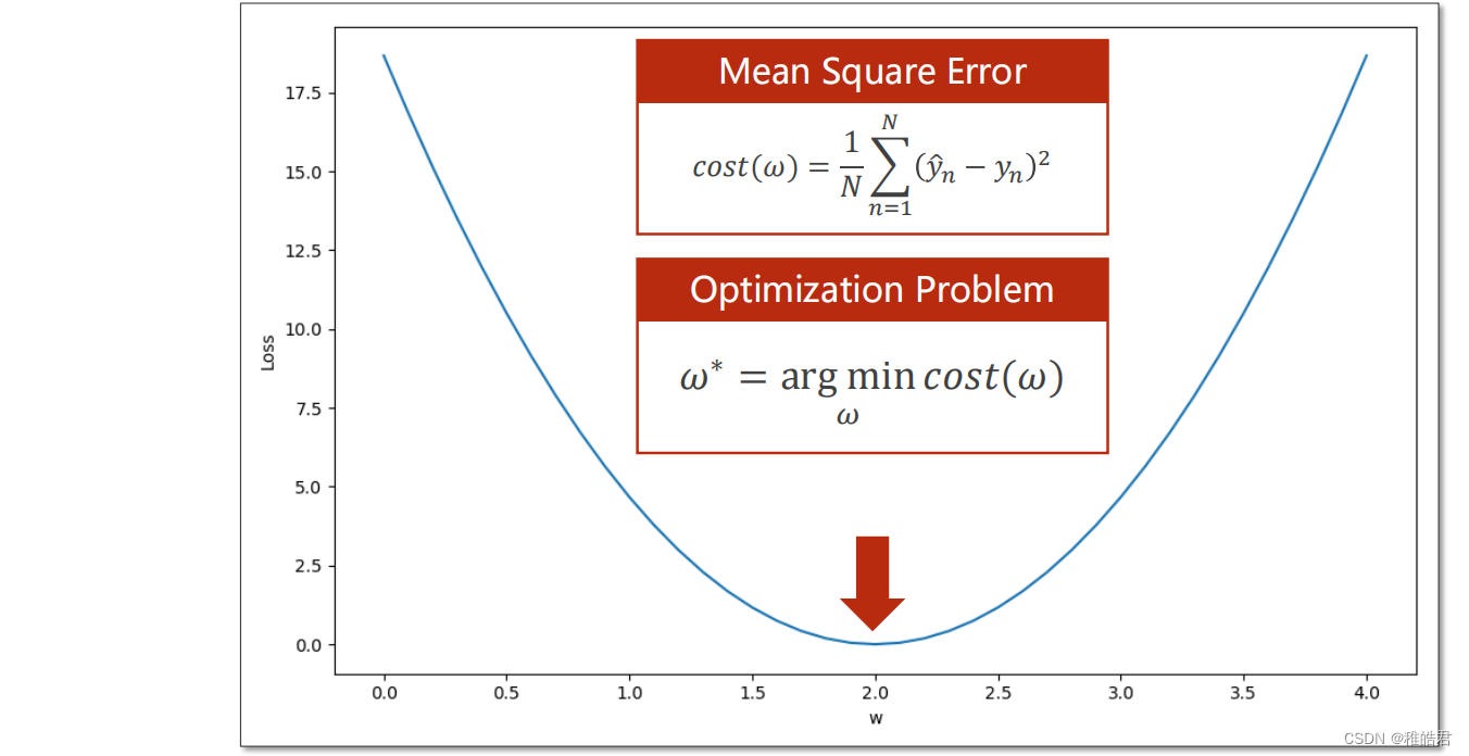
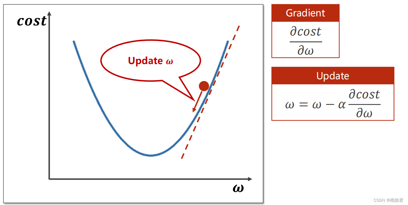
梯度下降

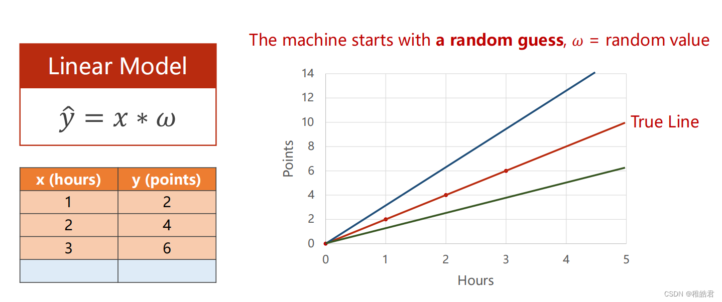
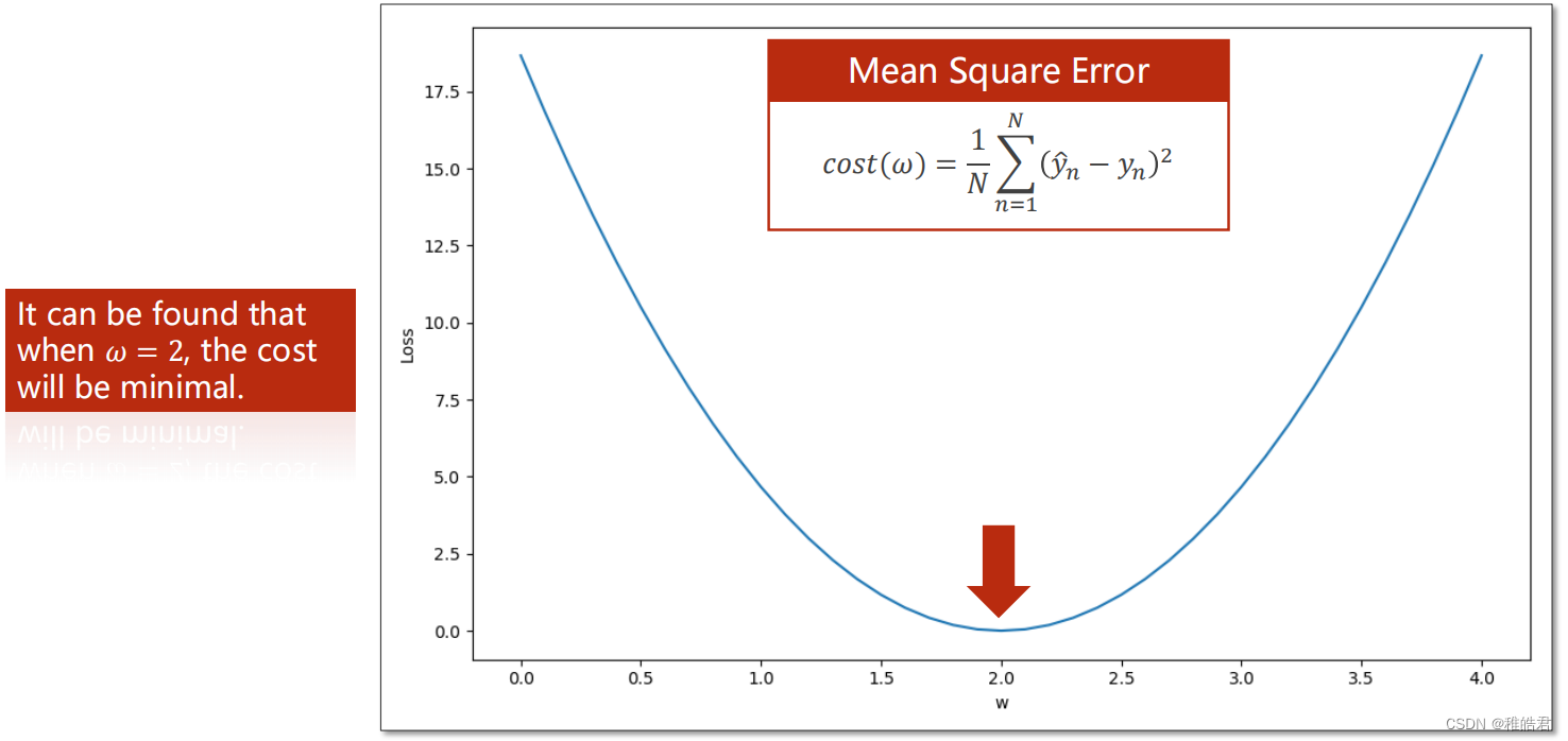
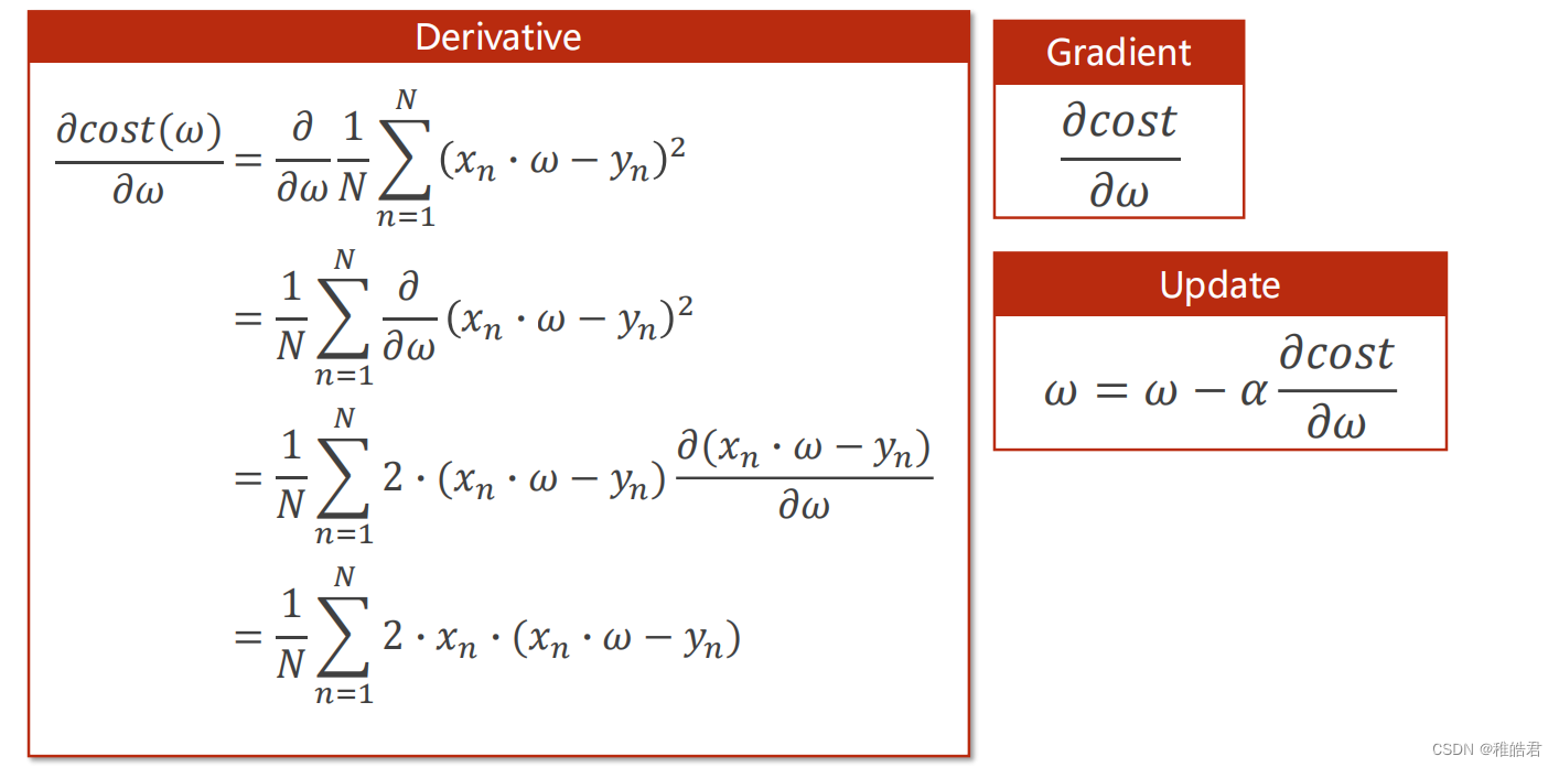
问题分析

编程实现

代码

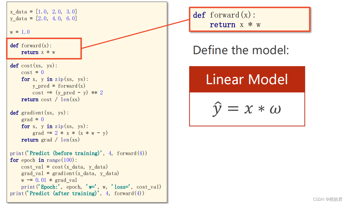
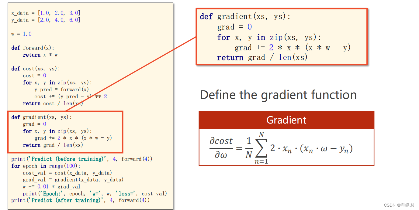
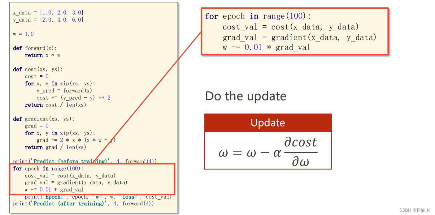
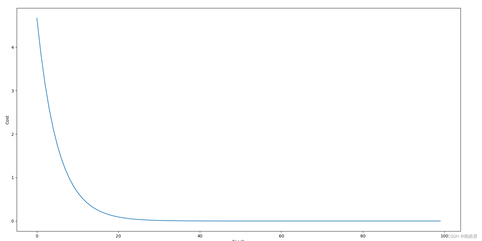
import matplotlib.pyplot as plt

# 训练集数据
x_data = [1.0, 2.0, 3.0]
y_data = [2.0, 4.0, 6.0]

# 设置初始权重猜测
w = 1.0

# 前馈计算
def forward(x):
    return x * w

# 计算损失
def cost(xs, ys):
    cost = 0
    for x, y in zip(xs, ys):
        y_pred = forward(x)
        cost += (y_pred - y) ** 2
    return cost / len(xs)

# 计算梯度
def gradien(xs, ys):
    grad = 0
    for x, y in zip(xs, ys):
        grad += 2 * x * (x * w - y)
    return grad / len(xs)

print('Predict(before training)', 4, forward(4))

# 存放每轮的数据
cost_list = []
epoch_list = []

# 训练过程
for epoch in range(100):  # 训练100轮
    cost_val = cost(x_data, y_data)
    grad_val = gradien(x_data, y_data)   # 更新梯度
    w -= 0.01 * grad_val    # 0.01 学习率
    print('Epoch:', epoch, 'w = ', w, 'loss = ', cost_val)
    cost_list.append(cost_val)
    epoch_list.append(epoch)

print('Predict(after training)', 4, forward(4))

# 绘图展示
plt.plot(epoch_list, cost_list)
plt.xlabel('Epoch')
plt.ylabel('Cost')
plt.show()

1
2
3
4
5
6
7
8
9
10
11
12
13
14
15
16
17
18
19
20
21
22
23
24
25
26
27
28
29
30
31
32
33
34
35
36
37
38
39
40
41
42
43
44
45
46
47
48
49
50
51

实现效果

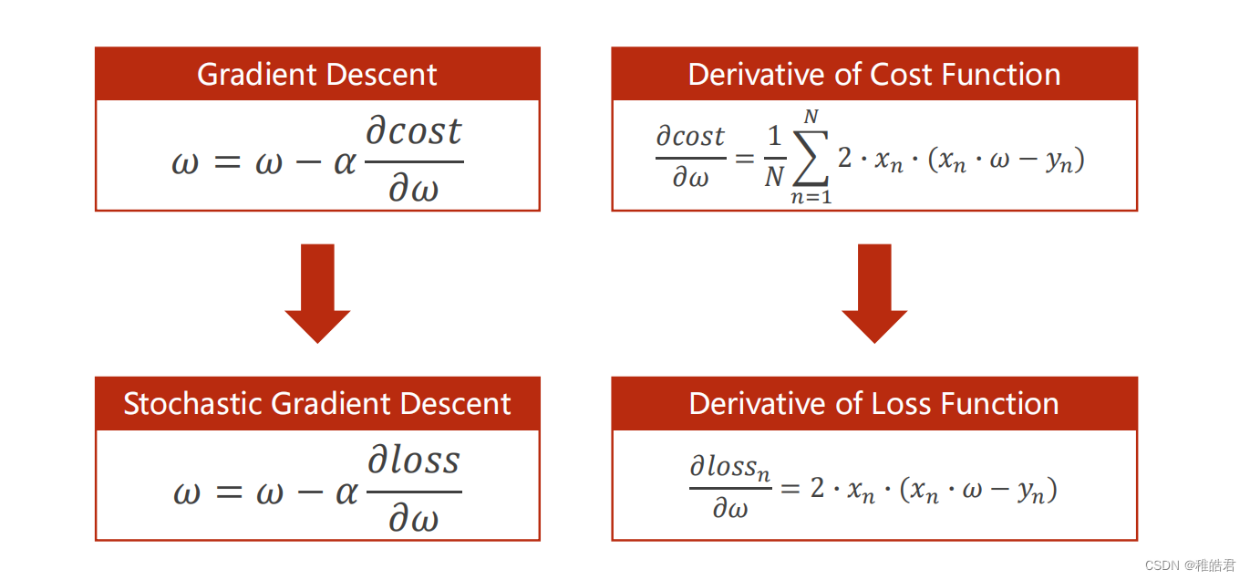
随机梯度下降

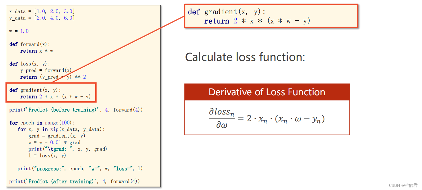
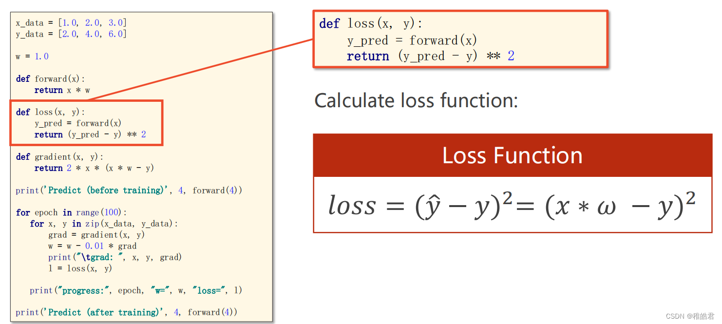
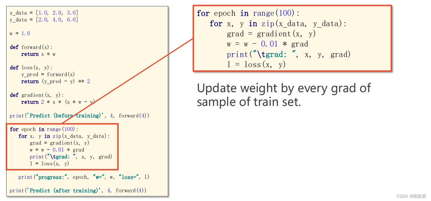
使用随机梯度下降对上述问题进行求解，随机梯度下降法和梯度下降法的主要区别在于：
1、损失函数由计算所有训练数据的损失，更改为计算一个训练数据的损失。
2、梯度函数由计算所有训练数据的梯度，更改为计算一个训练数据的梯度。

问题分析

编程实现

代码

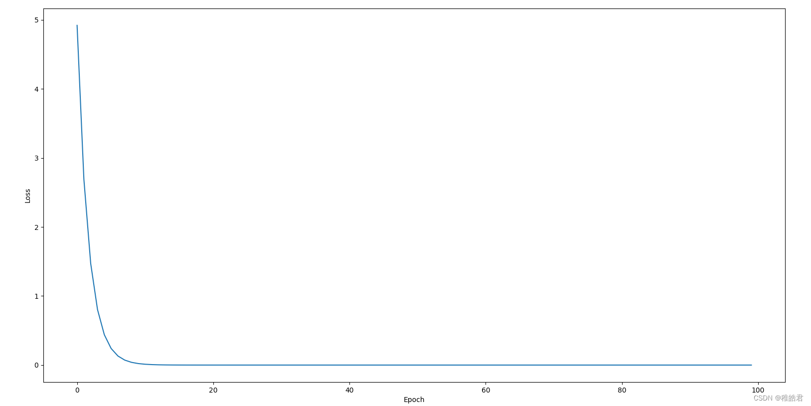
import matplotlib.pyplot as plt

# 训练集数据
x_data = [1.0, 2.0, 3.0]
y_data = [2.0, 4.0, 6.0]

# 设置初始权重猜测
w = 1.0

# 前馈计算
def forward(x):
    return x * w

# 计算损失
def loss(x, y):
    y_pred = forward(x)
    return (y_pred - y) ** 2

# 计算梯度
def gradien(x, y):
    return 2 * x * (x * w - y)

print('Predict(before training)', 4, forward(4))

# 存放每轮的数据
loss_list = []
epoch_list = []

# 训练过程
for epoch in range(100):  # 训练100轮
    for x, y in zip(x_data, y_data):
        grad = gradien(x, y)
        w = w - 0.01 * grad
        print('\tgrad:', x, y, grad)
        l = loss(x, y)
    epoch_list.append(epoch)
    loss_list.append(l)

print('Predict(after training)', 4, forward(4))

# 绘图展示
plt.plot(epoch_list, loss_list)
plt.xlabel('Epoch')
plt.ylabel('Loss')
plt.show()

1
2
3
4
5
6
7
8
9
10
11
12
13
14
15
16
17
18
19
20
21
22
23
24
25
26
27
28
29
30
31
32
33
34
35
36
37
38
39
40
41
42
43
44
45
46

实现效果

参考资料

传送门梯度下降算法