Optuna学习博客

介绍

Optuna就是一个能够进行调整超参数的框架，它能够将自动调整超参数以及能够将超参数优化过程可视化，方便保存，分析。可拓展性较强，减枝的优点。
剪枝操作会根据当前中间结果判断是否还需要进行下去。

optuna的优化程序具体有三个组成部分。

• objective，负责定义优化函数以及按照制定超参数的数值范围
• trial，对应着objective的执行（包括参数以及执行过程）
• study，负责管理优化，确定优化方式，实验总次数，时间等结果的实例（对象）

我们一般在objective函数中放置我们所需要优化的函数（确定优化目标）
下列以文档中给出的例子为参考。（主要针对不同模型的参数进行设置，所以在objective里面设置即可）如果有其他的需求可以参考官方文档。

使用案例

机器学习调整参数+优化历史进行可视化

import optuna
import sklearn
from sklearn.ensemble import RandomForestRegressor
from sklearn.datasets import load_digits
# Define an objective function to be minimized.
def objective(trial):

    # Invoke suggest methods of a Trial object to generate hyperparameters.
    # 确定优化模型的名称/种类
    regressor_name = trial.suggest_categorical('classifier', ['SVR', 'RandomForest'])
    if regressor_name == 'SVR':
        # 放置参数
        svr_c = trial.suggest_loguniform('svr_c', 1e-10, 1e10, log=True)
        regressor_obj = sklearn.svm.SVR(C=svr_c)
    else:
        rf_max_depth = trial.suggest_int('rf_max_depth', 2, 32)
        regressor_obj = RandomForestRegressor(max_depth=rf_max_depth)

    X, y = load_digits(return_X_y=True)
    X_train, X_val, y_train, y_val = sklearn.model_selection.train_test_split(X, y, random_state=0)

    regressor_obj.fit(X_train, y_train)
    y_pred = regressor_obj.predict(X_val)

    error = sklearn.metrics.mean_squared_error(y_val, y_pred)
     # An objective value linked with the Trial object.
    return error 
 # Create a new study.
study = optuna.create_study(study_name='svm_test_optuna', direction='minimize') 
# 这里可以选择迭代的次数n_trials
# Invoke optimization of the objective function.
study.optimize(objective, n_trials=10) 
# 在这一步的时候需要运用pip install -U plotly>=4.0.0去安装plotly这个库进行每个trial的可视化
# 可视化的时候需要用下列的表达式去判断
print(optuna.visualization.is_available())
fig = optuna.visualization.plot_optimization_history(study)
fig.show()
print(study.best_params) # 最优参数
print(study.best_value) # 最优的loss/优化目标数值
1
2
3
4
5
6
7
8
9
10
11
12
13
14
15
16
17
18
19
20
21
22
23
24
25
26
27
28
29
30
31
32
33
34
35
36
37
38
39

返回的结果如下所示。

True
{‘classifier’: ‘SVR’, ‘svr_c’: 10748891.080318237}
0.5439382462559595

绘制各 trail单次实验次数的学习曲线（MLP模型为例子）

import optuna
from matplotlib import pyplot as plt
from sklearn.datasets import load_iris
from sklearn.model_selection import train_test_split
from optuna.visualization import plot_intermediate_values

import torch.nn as nn
import torch.optim as optim
from torch.utils.data import Dataset, DataLoader

# 加载Iris数据集
iris = load_iris()
X, y = iris.data, iris.target
X = X.astype(float)
y = y.astype(int)
# 划分训练集和验证集
X_train, X_val, y_train, y_val = train_test_split(X, y, test_size=0.2, random_state=42)


# 定义自定义数据集类
class CustomDataset(Dataset):
    def __init__(self, data, target):
        self.data = data
        self.target = target

    def __len__(self):
        return len(self.data)

    def __getitem__(self, idx):
        x = self.data[idx]
        y = self.target[idx]
        return x, y

# 单层MLP
class mlp_model(nn.Module):
    def __init__(self, input_size):
        super(mlp_model, self).__init__()
        self.linear = nn.Linear(input_size, 1)
        self.relu = nn.ReLU()

    def forward(self, x):
        x = x.float()
        x = self.relu(x)
        out = self.linear(x)
        return out

# 定义目标函数
def objective(trial):
    # 超参数搜索空间
    learning_rate = trial.suggest_loguniform('learning_rate', 1e-5, 1e-1)

    # 创建模型和数据加载器
    model = mlp_model(input_size=X_train.shape[1])
    criterion = nn.HingeEmbeddingLoss()
    optimizer = optim.SGD(model.parameters(), lr=learning_rate)

    train_dataset = CustomDataset(X_train, y_train)
    train_loader = DataLoader(train_dataset, batch_size=16, shuffle=True)

    num_epochs = 50
    train_loss = []

    for epoch in range(num_epochs):
        model.train()
        epoch_loss = 0.0

        for batch_x, batch_y in train_loader:
            optimizer.zero_grad()
            output = model(batch_x)
            loss = criterion(output.squeeze(), batch_y.float())
            loss.backward()
            optimizer.step()

            epoch_loss += loss.item()

        train_loss.append(epoch_loss / len(train_loader))

        trial.report(epoch_loss, epoch)

        if trial.should_prune():
            raise optuna.exceptions.TrialPruned()

    return train_loss[-1]

# 创建Optuna学习实例
study = optuna.create_study(direction='minimize')
study.optimize(objective, n_trials=10)

# 绘制中间值图
plot_intermediate_values(study).show()
#

1
2
3
4
5
6
7
8
9
10
11
12
13
14
15
16
17
18
19
20
21
22
23
24
25
26
27
28
29
30
31
32
33
34
35
36
37
38
39
40
41
42
43
44
45
46
47
48
49
50
51
52
53
54
55
56
57
58
59
60
61
62
63
64
65
66
67
68
69
70
71
72
73
74
75
76
77
78
79
80
81
82
83
84
85
86
87
88
89
90
91
92

结果如图所示。（呈现交互式结果）

设置优化参数

• suggest_categorical(name, choices) 设置模型的名称或者为种类
• suggest_discrete_uniform(name, low, high, q) 设置离散类型变量的区间以及步长
• suggest_float(name, low, high, *[, step, log]) 设置浮点类型数据的区间和步长
• suggest_int(name, low, high[, step, log]) 设置整形类型数据的区间和步长
• suggest_loguniform(name, low, high) 设置连续类型数据的区间和步长（一般用这个设置学习率）
  suggest_uniform(name, low, high) 设置连续类型数据的区间和步长

原文介绍如下所示。
具体可以参考下列链接。有关于设置参数的optuna搜索结果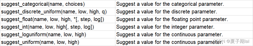

查看优化参数参数以及结果

主要是通过study的参数查询即可。

• study.best_params（最优的参数）
• best_trial（最优的实验次数）
• best_valye（最优的loss/优化目标的值）

参考资料

或许是东半球最好用的超参数优化框架： Optuna 简介
Optuna: 一个超参数优化框架（官方中文文档）
Optimize Your Optimization（官方网站）
Optuna: 一个超参数优化框架（官方英文文档）