强化学习Q-learning实践

1. 引言

前篇文章介绍了强化学习系统红的基本概念和重要组成部分，并解释了Q-learning算法相关的理论知识。本文的目标是在Python3中实现该算法，并将其应用于实际的实验中。
闲话少说，我们直接开始吧！

2. Taxi-v3 Env

为了使本文具有实际具体的意义，特意选择了一个简单而基本的环境，可以让大家充分欣赏Q-learning算法的优雅。我们选择的环境是OpenAI Gym的Taxi-v3，该环境简单明了，是强化学习RL领域的优秀入门样例。实际上Taxi-v3由一个grid map组成，如下图示：

其中，该环境下的agent是一名出租车司机，他必须接客户（红色小人）并将其送到目的地（图中的小房子）。

3. States

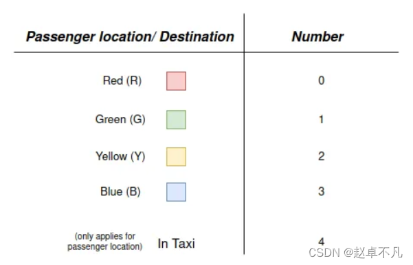
一版来说，States的作用如下 (1) 确定action（2）计算执行action的奖励reward（3）计算到下一状态的转换所需的信息。

观察上图，我们的网格grid map的大小为5x5，所以出租车所有可能的选择有25个。除此之外，等待接车的乘客可以在四个可能的接车点（标记为Y、R、G、B）处等待当然也可以在出租车里，所以乘客所有可能的选择有(4+1)个；最后，乘客的目的地在(Y、R、G、B)四个中的一个，所以乘客的目的地共有4个选择，图示如下：

综上，我们用以下向量表示States：

State = [x_pos_taxi, y_pos_taxi, pos_passenger, dest_passenger]

进而，我们agent的States一共有5X5X5X4=500个，可以被编码为0到499之间的整数。其实，实际可用的状态的数量略小于500，例如，乘客将永远不会有相同的乘车点和目的地。由于建模的复杂性，我们通常关注完整的状态空间。

4. 举个栗子

上述文字讲完后，有些同学还是有很多不理解的东东，那我们来找个中间过程来看看，如下：

上图中，STATE:(2,1,0,1)表示，当前出租车在grid map中的第二行第一列，同时乘客的状态选择为0表示位于乘客位于红色格子里等待乘车，同时乘客的目的地状态选择为1表示乘客的目的地为绿色格子。
进而，下图中的STATE:(3,4,4,0)表示，当前出租车在grid map中的第三行第四列，同时乘客的状态选择为4表示此时乘客位于出租车里，同时乘客的目的地状态选择为0 ，表示乘客的目的地为红色格子。

看到这里的童鞋，请仔细理解上述两个例子。

5. Action space

至于该环境Env下agent的动作空间Action space，我们可以想象，代理agent可以使用以下离散动作来与环境交互：向前、向后、向右、向左、接乘客和送乘客。这使得总共有6个可能的动作，这些动作依次以0到5的数字编码，以便于编程。动作和数字之间的对应关系如图1所示。

6. Rewards

至于agent执行的每一步action所获得的奖励reward，做如下约定：

• 移动：-1, 表示每一步都会受到一点惩罚，以鼓励从出发地到目的地走最短的路。
• 错误运送：-10， 表示当乘客被送到到错误的位置时，乘客自然会不高兴，所以惩罚大一些是合适的。
• 成功送达:20，表示出租车司机成功完成了任务，鼓励相应的行为，因此产生了正向的reward。

7. Initialization

在数学上定义了这个问题之后，我们接着将着手用代码实现。首先，我们安装必要的库，然后导入它们。显然，我们需要安装gym 环境。除此之外，我们只需要一些可视化的东西和常见的数据处理库。

"""install libraries"""
!pip install cmake 'gym[atari]' scipy pygame

"""Import libraries"""
import gym
import numpy as np
import matplotlib.pyplot as plt
import random
from IPython.display import clear_output
from time import sleep
from matplotlib import animation
1
2
3
4
5
6
7
8
9
10
11

接着，我们使用以下代码来创建和渲染Taxi-v3环境。

"""Initialize and validate the environment"""
env = gym.make("Taxi-v3", render_mode="rgb_array").env
state, _ = env.reset()

# Print dimensions of state and action space
print("State space: {}".format(env.observation_space))
print("Action space: {}".format(env.action_space))

# Sample random action
action = env.action_space.sample(env.action_mask(state))
next_state, reward, done, _, _ = env.step(action)

# Print output
print("State: {}".format(state))
print("Action: {}".format(action))
print("Action mask: {}".format(env.action_mask(state)))
print("Reward: {}".format(reward))

# Render and plot an environment frame
frame = env.render()
plt.imshow(frame)
plt.axis("off")
plt.show()
1
2
3
4
5
6
7
8
9
10
11
12
13
14
15
16
17
18
19
20
21
22
23

结果如下：

8. 测试随机agent

在上述环境Env按照预期开始工作后，此时我们可以随机让代理疯狂运行了。我们不妨让我们的agent在任何时刻都会采取随机行动，来看看会产生怎样的效果。

"""Simulation with random agent"""
epoch = 0
num_failed_dropoffs = 0
experience_buffer = []
cum_reward = 0

done = False

state, _ = env.reset()

while not done:
    # Sample random action
    "Action selection without action mask"
    action = env.action_space.sample()

    "Action selection with action mask"
    #action = env.action_space.sample(env.action_mask(state))

    state, reward, done, _, _ = env.step(action)
    cum_reward += reward

    # Store experience in dictionary
    experience_buffer.append({
        "frame": env.render(),
        "episode": 1,
        "epoch": epoch,
        "state": state,
        "action": action,
        "reward": cum_reward,
        }
    )

    if reward == -10:
        num_failed_dropoffs += 1

    epoch += 1

# Run animation and print console output
run_animation(experience_buffer)

print("# epochs: {}".format(epoch))
print("# failed drop-offs: {}".format(num_failed_dropoffs))
1
2
3
4
5
6
7
8
9
10
11
12
13
14
15
16
17
18
19
20
21
22
23
24
25
26
27
28
29
30
31
32
33
34
35
36
37
38
39
40
41
42

运行上述代码后，得到结果如下：

为什么要看完上述冗长的动画？好吧，这确实给人一种印象，一个未经训练的RL模型下的agent是如何表现的，以及需要多长时间才能获得有意义的reward。

9. 训练agent

接着，我们来尝试训练我们的agent，我们知道Q值是在进行观测之后使用以下等式进行更新的。

请注意，对于500个状态和6个动作，我们必须填写一个大小为500*6=3000的Q表，每个状态-动作二元组需要多次观察才能学到有用的知识。相应的训练代码如下：

"""Training the agent"""
q_table = np.zeros([env.observation_space.n, env.action_space.n])

# Hyperparameters
alpha = 0.1  # Learning rate
gamma = 1.0  # Discount rate
epsilon = 0.1  # Exploration rate
num_episodes = 10000  # Number of episodes

# Output for plots
cum_rewards = np.zeros([num_episodes])
total_epochs = np.zeros([num_episodes])

for episode in range(1, num_episodes+1):
    # Reset environment
    state, info = env.reset()
    epoch = 0 
    num_failed_dropoffs = 0
    done = False
    cum_reward = 0

    while not done:
        
        if random.uniform(0, 1) < epsilon:
            "Basic exploration [~0.47m]"
            action = env.action_space.sample() # Sample random action (exploration)
            
            "Exploration with action mask [~1.52m]"
          # action = env.action_space.sample(env.action_mask(state)) "Exploration with action mask"
        else:      
            "Exploitation with action mask [~1m52s]"
           # action_mask = np.where(info["action_mask"]==1,0,1) # invert
           # masked_q_values = np.ma.array(q_table[state], mask=action_mask, dtype=np.float32)
           # action = np.ma.argmax(masked_q_values, axis=0)

            "Exploitation with random tie breaker [~1m19s]"
          #  action = np.random.choice(np.flatnonzero(q_table[state] == q_table[state].max()))
            
            "Basic exploitation [~47s]"
            action = np.argmax(q_table[state]) # Select best known action (exploitation)
 
        next_state, reward, done, _ , info = env.step(action) 

        cum_reward += reward
        
        old_q_value = q_table[state, action]
        next_max = np.max(q_table[next_state])
        
        new_q_value = (1 - alpha) * old_q_value + alpha * (reward + gamma * next_max)
        
        q_table[state, action] = new_q_value
        
        if reward == -10:
            num_failed_dropoffs += 1

        state = next_state
        epoch += 1
        
        total_epochs[episode-1] = epoch
        cum_rewards[episode-1] = cum_reward

    if episode % 100 == 0:
        clear_output(wait=True)
        print(f"Episode #: {episode}")

print("\n")
print("===Training completed.===\n")

# Plot reward convergence
plt.title("Cumulative reward per episode")
plt.xlabel("Episode")
plt.ylabel("Cumulative reward")
plt.plot(cum_rewards)
plt.show()

# Plot epoch convergence
plt.title("# epochs per episode")
plt.xlabel("Episode")
plt.ylabel("# epochs")
plt.plot(total_epochs)
plt.show()
1
2
3
4
5
6
7
8
9
10
11
12
13
14
15
16
17
18
19
20
21
22
23
24
25
26
27
28
29
30
31
32
33
34
35
36
37
38
39
40
41
42
43
44
45
46
47
48
49
50
51
52
53
54
55
56
57
58
59
60
61
62
63
64
65
66
67
68
69
70
71
72
73
74
75
76
77
78
79
80
81

在2000个episode 之后，我们似乎学到了一个相当好的模型，如下：

上图图像中，横坐标表示我们一共训练了10000个Episode，纵坐标表示每一个Episode下，出租车司机将乘客送达目的地所需要的移动步数epochs。

10. 验证训练效果

最后，让我们看看我们的模型学到了什么。根据我们所处的状态，我们在Q表中查找相应的Q值（即，每个状态对应于动作的六个值），并选择具有最高相关Q值的动作。代码如下：

"""Test policy performance after training"""

num_epochs = 0
total_failed_deliveries = 0
num_episodes = 1
experience_buffer = []
store_gif = True

for episode in range(1, num_episodes+1):
    # Initialize experience buffer

    my_env = env.reset()
    state = my_env[0]
    epoch = 1 
    num_failed_deliveries =0
    cum_reward = 0
    done = False

    while not done:
        action = np.argmax(q_table[state])
        state, reward, done, _, _ = env.step(action)
        cum_reward += reward

        if reward == -10:
            num_failed_deliveries += 1

        # Store rendered frame in animation dictionary
        experience_buffer.append({
            'frame': env.render(),
            'episode': episode,
            'epoch': epoch,
            'state': state,
            'action': action,
            'reward': cum_reward
            }
        )

        epoch += 1

    total_failed_deliveries += num_failed_deliveries
    num_epochs += epoch

    if store_gif:
        store_episode_as_gif(experience_buffer)

# Run animation and print output
run_animation(experience_buffer)

# Print final results
print("\n") 
print(f"Test results after {num_episodes} episodes:")
print(f"Mean # epochs per episode: {num_epochs / num_episodes}")
print(f"Mean # failed drop-offs per episode: {total_failed_deliveries / num_episodes}")
1
2
3
4
5
6
7
8
9
10
11
12
13
14
15
16
17
18
19
20
21
22
23
24
25
26
27
28
29
30
31
32
33
34
35
36
37
38
39
40
41
42
43
44
45
46
47
48
49
50
51
52
53

结果如下:

可以看到，在执行了足够多的迭代之后，我们可以发现出租车总是直接驶向乘客，走最短的路到达目的地，并成功地将乘客放下。

11. 总结

本文通过具体的应用，来对前篇Q-learning的理论知识用代码进行了详细的说明，主要通过业内知名的Taxi-v3环境进行了讲解，并给出了完整的代码示例。

您学废了嘛？