神经网络和深度学习-处理多维特征的输入

处理多维特征的输入

前面有两个数据集，一个回归，一个分类。

在回归中输出y属于实数，而在分类中输出y属于一个离散的集合

例如在糖尿病分类的数据集中Diabetes Dataset，每一行作为一个sample（样本），每一列作为一个feature（特征）

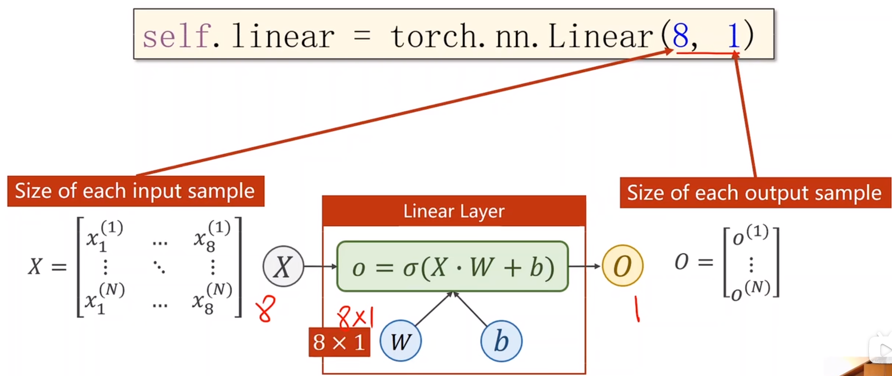
之前我们在一个维度上的logistic回归模型为

现在我们要拓展到8个维度上面，每一个特征的的取值都要和权重进行相乘

之后再将XW进行展开，并进行sigmoid函数

接下来我们看一下mini-batch的情况对于1-N个样本都要求sigmoid，他们都是按照向量计算的函数

[ y ^ ( 1 ) ⋮ y ^ ( N ) ] = [ σ ( z ( 1 ) ) ⋮ σ ( z ( N ) ) ] = σ ( [ z ( 1 ) ⋮ z ( N ) ] ) \left[

\right]=\left[\right]=\sigma\left(\left[\right]\right) ⎣⎢⎡​y^​(1)⋮y^​(N)​⎦⎥⎤​=⎣⎢⎡​σ(z(1))⋮σ(z(N))​⎦⎥⎤​=σ⎝⎜⎛​⎣⎢⎡​z(1)⋮z(N)​⎦⎥⎤​⎠⎟⎞​

Z从第1个样本到第8个样本计算的时候，z1等于第一个样本的x1到x8 乘上权重，在加偏置

z ( 1 ) = [ x 1 ( 1 ) ⋯ x 8 ( 1 ) ] [ ω 1 ⋮ ω 8 ] + b z ( N ) = [ x 1 ( N ) ⋯ x 8 ( N ) ] [ ω 1 ⋮ ω 8 ] + b z^{(1)}=\left[

\right]\left[\right]+b\\z^{(N)}=\left[\right]\left[\right]+b z(1)=[x1(1)​​⋯​x8(1)​​]⎣⎢⎡​ω1​⋮ω8​​⎦⎥⎤​+bz(N)=[x1(N)​​⋯​x8(N)​​]⎣⎢⎡​ω1​⋮ω8​​⎦⎥⎤​+b

同时将Z看作一组向量的运算

[ z ( 1 ) ⋮ z ( N ) ] = [ x 1 ( 1 ) … x 8 ( 1 ) ⋮ ⋱ ⋮ x 1 ( N ) … x 8 ( N ) ] [ ω 1 ⋮ ω 8 ] + [ b ⋮ b ] \left[

\right]=\left[\right]\left[\right]+\left[\right] ⎣⎢⎡​z(1)⋮z(N)​⎦⎥⎤​=⎣⎢⎢⎡​x1(1)​⋮x1(N)​​…⋱…​x8(1)​⋮x8(N)​​⎦⎥⎥⎤​⎣⎢⎡​ω1​⋮ω8​​⎦⎥⎤​+⎣⎢⎡​b⋮b​⎦⎥⎤​

我们来看一下转换为向量化计算的完整结构图，提高运行速度

我们再来看一下他的代码形式，输入的x维度为8，输出的z维度为1

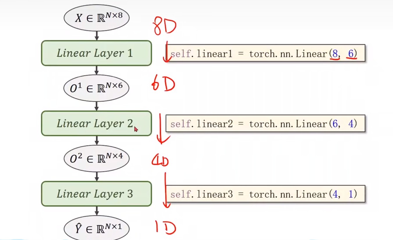
假如我们需要一个（8，2）的维度，输出变成了两个维度，只需要在后面增加一个（2，1）的维度，就可以降到1维

在神经网络中我们就可以进行转换维度，但转入更高的维度，更多的隐层，虽然能提取更多特征，但是相应的也会出现更多的噪声，我们应该提高的是泛化能力

我们下面结合糖尿病分类的数据集中Diabetes Dataset来看，x1-x8是糖尿病患者相应的指标，y代表病情是否会在一年之后加重

我们继续按照四个模块来进行代码分析

准备数据：首先我们来看一下数据的读取

定义模型：我们采用多个线性模型来定义模型

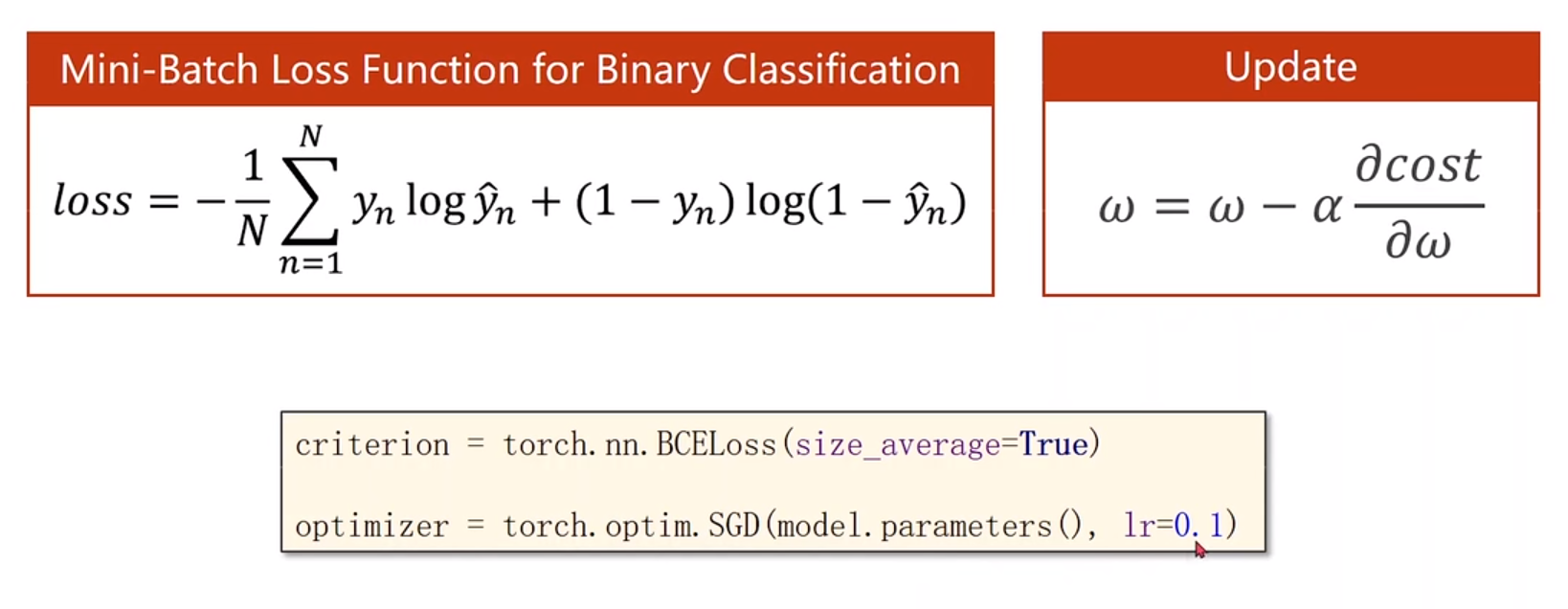
构造损失和优化器：与之前的logistic回归之中并没有什么变化，学习率改为0.1进行训练

训练周期：在这里并没有使用mini-batch

我们也可以选择多种不同的激活函数

详细的内容我们可以查询文档

https://pytorch.org/docs/stable/index.html

比如我们想要改变激活函数Relu时，只需要改变一个地方，但后面如果要计算预测Y时也需要改成sigmoid函数

关于数据集的下载，我们可以到下面的网站进行下载，该数据集需要和源码放入同一个文件夹

diabetes.csv.gz

完整代码如下，这里训练epoch设置为1000，但并没有得到拟合的损失

import numpy as np
import torch
import matplotlib.pyplot as plt

# prepare dataset
xy = np.loadtxt('diabetes.csv.gz', delimiter=',', dtype=np.float32)
x_data = torch.from_numpy(xy[:, :-1])  # 第一个‘：’是指读取所有行，第二个‘：’是指从第一列开始，最后一列不要
y_data = torch.from_numpy(xy[:, [-1]])  # [-1] 最后得到的是个矩阵


# design model using class


class Model(torch.nn.Module):
    def __init__(self):
        super(Model, self).__init__()
        self.linear1 = torch.nn.Linear(8, 6)  # 输入数据x的特征是8维，x有8个特征
        self.linear2 = torch.nn.Linear(6, 4)
        self.linear3 = torch.nn.Linear(4, 1)
        self.sigmoid = torch.nn.Sigmoid()  # 将其看作是网络的一层，而不是简单的函数使用

    def forward(self, x):
        x = self.sigmoid(self.linear1(x))
        x = self.sigmoid(self.linear2(x))
        x = self.sigmoid(self.linear3(x))  # y hat
        return x


model = Model()

# construct loss and optimizer
# criterion = torch.nn.BCELoss(size_average = True)
criterion = torch.nn.BCELoss(reduction='mean')
optimizer = torch.optim.SGD(model.parameters(), lr=0.1)

epoch_list = []
loss_list = []
# training cycle forward, backward, update
for epoch in range(1000):
    y_pred = model(x_data)
    loss = criterion(y_pred, y_data)
    print(epoch, loss.item())
    epoch_list.append(epoch)
    loss_list.append(loss.item())

    optimizer.zero_grad()
    loss.backward()

    optimizer.step()

plt.plot(epoch_list, loss_list)
plt.ylabel('loss')
plt.xlabel('epoch')
plt.show()
1
2
3
4
5
6
7
8
9
10
11
12
13
14
15
16
17
18
19
20
21
22
23
24
25
26
27
28
29
30
31
32
33
34
35
36
37
38
39
40
41
42
43
44
45
46
47
48
49
50
51
52
53
54

图像显示为：

如果我们将epoch改为100000时，拟合到一定的程度，但还是可以继续进行下去

import numpy as np
import torch
import matplotlib.pyplot as plt

# prepare dataset
xy = np.loadtxt('diabetes.csv.gz', delimiter=',', dtype=np.float32)
x_data = torch.from_numpy(xy[:, :-1])  # 第一个‘：’是指读取所有行，第二个‘：’是指从第一列开始，最后一列不要
y_data = torch.from_numpy(xy[:, [-1]])  # [-1] 最后得到的是个矩阵


# design model using class


class Model(torch.nn.Module):
    def __init__(self):
        super(Model, self).__init__()
        self.linear1 = torch.nn.Linear(8, 6)  # 输入数据x的特征是8维，x有8个特征
        self.linear2 = torch.nn.Linear(6, 4)
        self.linear3 = torch.nn.Linear(4, 1)
        self.sigmoid = torch.nn.Sigmoid()  # 将其看作是网络的一层，而不是简单的函数使用

    def forward(self, x):
        x = self.sigmoid(self.linear1(x))
        x = self.sigmoid(self.linear2(x))
        x = self.sigmoid(self.linear3(x))  # y hat
        return x


model = Model()

# construct loss and optimizer
# criterion = torch.nn.BCELoss(size_average = True)
criterion = torch.nn.BCELoss(reduction='mean')
optimizer = torch.optim.SGD(model.parameters(), lr=0.1)

epoch_list = []
loss_list = []
# training cycle forward, backward, update
for epoch in range(100000):
    y_pred = model(x_data)
    loss = criterion(y_pred, y_data)
    print(epoch, loss.item()) 
    epoch_list.append(epoch)
    loss_list.append(loss.item())

    optimizer.zero_grad()
    loss.backward()

    optimizer.step()

plt.plot(epoch_list, loss_list)
plt.ylabel('loss')
plt.xlabel('epoch')
plt.show()
1
2
3
4
5
6
7
8
9
10
11
12
13
14
15
16
17
18
19
20
21
22
23
24
25
26
27
28
29
30
31
32
33
34
35
36
37
38
39
40
41
42
43
44
45
46
47
48
49
50
51
52
53
54

图像显示为：

如果想查看某些层的参数，以神经网络的第一层参数为例，可按照以下方法进行

# 参数说明
# 第一层的参数：
layer1_weight = model.linear1.weight.data
layer1_bias = model.linear1.bias.data
print("layer1_weight", layer1_weight)
print("layer1_weight.shape", layer1_weight.shape)
print("layer1_bias", layer1_bias)
print("layer1_bias.shape", layer1_bias.shape)
1
2
3
4
5
6
7
8