-
1.1 极限的概念
1.1 极限的概念
引言
- 在物理实验中,如果涉及到测量,那么误差总是存在的。误差是在正确实验的情况下实验测量值与理论值之间的差值。
- 如果理论是正确的并且使用更精密的实验仪器或改进实验方法,那么测量值就会更加接近理论值,这时我们可以认为理论值是测量值的极限。
- 物理中用误差来刻画理论值和测量值之间的差距,数学是现实的抽象表述,数学中通常使用希腊字母
ε
{\varepsilon}
ε
(英文发音Epsilon)来表述一个变量与另一个固定实数之间的差值,差值越小,两者越接近,如果这个差值可以任意小,那么这个变量的极限就是这个固定实数。
1.1.1 数列的极限
引例
举一个例子来更加清楚地理解极限。
- 从前有一个愚公想要搬走门前的一座大山。

简化如下

- 第一代人比较努力,搬走了这座山的二分之一。

- 第二代人就不太努力了,只搬走了这座山剩下的二分之一。
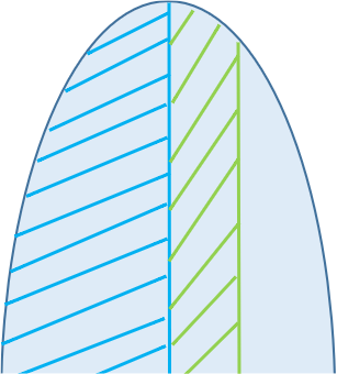
- 后面的每一代人都只搬走这座山剩余的二分之一。


-
观察图像可以发现他们移山的过程中每一代人搬走的越来越少,一直搬下去会越来越接近一整座山。
-
用数学模型来表示
第几代人 1 2 3 4 5 6 7 8 9 每一代人搬走的山 1/2 1/4 1/8 1/16 1/32 1/64 1/128 1/256 1/572 一共搬走的山 1/2 3/4 7/8 15/16 31/32 63/64 127/128 255/256 571/572 - 每一代人搬走的山视为数列的项,每一项越来越接近
0,而不会等于0,即数列项的极限值为0。 - 一共搬走的山视为数列的和,数列和越来越接近
1,而不会等于1,即数列和的极限值为1。
定义
数列的极限
如果对于任意给定的 ε > 0 \varepsilon>0 ε>0, 总存在正整数 N N N , 当 n > N n>N n>N 时, 恒有
∣ x n − a ∣ < ε \left|x_{n}-a\right|<\varepsilon ∣xn−a∣<ε成立, 则称常数 a a a 为数列 { x n } \left\{x_{n}\right\} {xn}当 n n n 趋于无穷时的极限,记为
lim n → ∞ x n = a \displaystyle\lim _{n \rightarrow \infty} x_{n}=a n→∞limxn=a
称数列收敛到 a a a,如果一个数列不收敛,则称它发散。几何意义
数列的图像在一维直线坐标轴上是散列点,如果数列是收敛的,那么随着 n → ∞ n \rightarrow \infty n→∞ ( n n n趋于无穷),这些点会向某一个位置靠拢。
例如数列 a n = n + 1 n a_{n}=\frac{n+1}{n} an=nn+1,如图所示, a n a_n an会逐渐向1靠拢。

lim n → ∞ x n = a \displaystyle\lim _{n \rightarrow \infty} x_{n}=a n→∞limxn=a :对于 a a a 点的任何 ε \varepsilon ε 邻域即开区间 ( a − ε , a + ε ) (a-\varepsilon, a+\varepsilon) (a−ε,a+ε), 一定存在 N N N,当 n > N n>N n>N 即第 N N N 项以后的点 x n x_{n} xn 都落在开区间 ( a − ε , a + ε ) (a-\varepsilon, a+\varepsilon ) (a−ε,a+ε)内, 而只有有限个 (最多有 N N N个) 在这区间之外。
注意
- ε \varepsilon ε是用来刻画 x n x_{n} xn 与 a a a 的接近程度, N N N 是用来刻画 n → ∞ n \rightarrow \infty n→∞ ( n n n趋于无穷)这个极限过程。
- 数列 { x n } \left\{x_{n}\right\} {xn}的极限是否存在, 如果存在极限值等于多少,与数列的前有限项无关。
典例:极限定义的应用
数列的通项为 a n = 1 n a_{n}=\frac{1}{n} an=n1, 证明 lim n → ∞ a n = 0 \displaystyle\lim _{n \rightarrow \infty} a_{n}=0 n→∞liman=0。
分析:利用数列极限的定义证明,当 n n n 大于某一个值时, a n a_{n} an和 0 0 0 的差值的绝对值小于任意给定大于 0 0 0的数。
证明:取任意 ε > 0 \varepsilon>0 ε>0,当 n > 1 ε n>\frac{1}{\varepsilon} n>ε1 时, 1 n < ε \frac{1}{n} < \varepsilon n1<ε,故 当 n > 1 ε n>\frac{1}{\varepsilon} n>ε1 时, 有 ∣ 1 n − 0 ∣ < ε \left|\frac{1}{n}-0\right|<\varepsilon n1−0 <ε 。从而 lim n → ∞ 1 n = 0 \displaystyle\lim _{n \rightarrow \infty} \frac{1}{n}=0 n→∞limn1=0 ,即 lim n → ∞ a n = 0 \displaystyle\lim _{n \rightarrow \infty} a_{n}=0 n→∞liman=0。
推论
如果理解了以上典例的证明过程,那么可以用类似的证明方法,根据数列极限的定义,得出三个常用的推论:
- lim n → ∞ x n = a ⇔ lim k → ∞ x 2 k − 1 = lim k → ∞ x 2 k = a \displaystyle\lim _{n \rightarrow \infty} x_{n}=a \Leftrightarrow \lim _{k \rightarrow \infty} x_{2 k-1}=\lim _{k \rightarrow \infty} x_{2 k}=a n→∞limxn=a⇔k→∞limx2k−1=k→∞limx2k=a。原数列的极限存在,则奇数列的极限等于偶数列的极限,且和原数列的极限值相等。
- 若 lim n → ∞ x n = a \displaystyle\lim _{n \rightarrow \infty} x_{n}=a n→∞limxn=a , 则 lim n → ∞ ∣ x n ∣ = ∣ a ∣ \displaystyle\lim _{n \rightarrow \infty}\left|x_{n}\right|=|a| n→∞lim∣xn∣=∣a∣ , 但反之不成立。
- lim n → ∞ x n = 0 \displaystyle\lim _{n \rightarrow \infty} x_{n}=0 n→∞limxn=0 的充分必要条件是 lim n → ∞ ∣ x n ∣ = 0 \displaystyle\lim _{n \rightarrow \infty}\left|x_{n}\right|=0 n→∞lim∣xn∣=0 。
三个推论的应用
推论1的应用:
(2006, 数三) lim n → ∞ ( n + 1 n ) ( − 1 ) n = \displaystyle\lim _{n \rightarrow \infty}\left(\frac{n+1}{n}\right)^{(-1)^{n}}= n→∞lim(nn+1)(−1)n=
解:当 n n n 为奇数时, x n = ( n + 1 n ) − 1 x_{n}=\left(\frac{n+1}{n}\right)^{-1} xn=(nn+1)−1 , lim n → ∞ x n = lim n → ∞ ( n + 1 n ) − 1 = 1 \displaystyle\lim _{n \rightarrow \infty} x_{n}=\lim _{n \rightarrow \infty}\left(\frac{n+1}{n}\right)^{-1}=1 n→∞limxn=n→∞lim(nn+1)−1=1
当 n n n 为偶数时, x n = n + 1 n x_{n}=\frac{n+1}{n} xn=nn+1 , lim n → ∞ x n = lim n → ∞ n + 1 n = 1 \displaystyle\lim _{n \rightarrow \infty} x_{n}=\lim _{n \rightarrow \infty} \frac{n+1}{n}=1 n→∞limxn=n→∞limnn+1=1
则 lim n → ∞ x n = lim n → ∞ ( n + 1 n ) ( − 1 ) n = 1 \displaystyle\lim _{n \rightarrow \infty} x_{n}=\lim _{n \rightarrow \infty}\left(\frac{n+1}{n}\right)^{(-1)^{n}}=1 n→∞limxn=n→∞lim(nn+1)(−1)n=1
推论2的应用:
设 lim n → ∞ a n = a \displaystyle\lim _{n \rightarrow \infty} a_{n}=a n→∞liman=a , 且 a ≠ 0 a \neq 0 a=0 , 则当 n n n 充分大时有(A)
A. ∣ a n ∣ > ∣ a ∣ 2 \left|a_{n}\right|>\frac{|a|}{2} ∣an∣>2∣a∣
B. ∣ a n ∣ < a 2 \left|a_{n}\right|<\frac{a}{2} ∣an∣<2a
C. a n > a − 1 n a_{n}>a-\frac{1}{n} an>a−n1
D. a n < a + 1 n a_{n}<\boldsymbol{a}+\frac{1}{n} an<a+n1解: lim n → ∞ a n = a \displaystyle\lim _{n \rightarrow \infty} a_{n}=a n→∞liman=a,则 lim n → ∞ ∣ a n ∣ = ∣ a ∣ \displaystyle\lim _{n \rightarrow \infty}\left|a_{n}\right|=|a| n→∞lim∣an∣=∣a∣,因为 ∣ a ∣ > ∣ a ∣ 2 \left|a\right|>\frac{|a|}{2} ∣a∣>2∣a∣ ,所以 ∣ a n ∣ > ∣ a ∣ 2 \left|a_{n}\right|>\frac{|a|}{2} ∣an∣>2∣a∣。
推论3的应用:
(1999, 数二)“对任意给定的 ε ∈ ( 0 , 1 ) \varepsilon \in(0,1) ε∈(0,1), 总存在正整数 N N N, 当 n ⩾ N n \geqslant N n⩾N 时, 恒有 ∣ x n − a ∣ ⩽ 2 ε \left|x_{n}-a\right| \leqslant 2 \varepsilon ∣xn−a∣⩽2ε” 是数列 { x n } \left\{x_{n}\right\} {xn} 收㪉于 a a a 的 ( C \color{Red}{C} C )
A.充分条件但非必要条件
B.必要条件但非充分条件
C.充分必要条件
D.既非必要也非充分条件
【解】本题没有直接用到推论3的结论,但证明过程类似。
- 由数列极限定义知, 如果数列 { x n } \left\{x_{n}\right\} {xn} 收敛于 a a a, 则对于任意给定的 ε > 0 \varepsilon>0 ε>0, 总存在正整数 N N N, 当 n > N n>N n>N 时, 恒有 ∣ x n − a ∣ < ε \left|x_{n}-a\right|<\varepsilon ∣xn−a∣<ε 成立,由于 ε < 2 ε \varepsilon<2 \varepsilon ε<2ε,必有 ∣ x n − a ∣ ⩽ 2 ε \left|x_{n}-a\right| \leqslant 2 \varepsilon ∣xn−a∣⩽2ε。得出必要条件。
- 对任意给定的 ε ∈ ( 0 , 1 ) \varepsilon \in(0,1) ε∈(0,1),总存在正整数 N N N,当 n ⩾ N n \geqslant N n⩾N 时, 恒有 ∣ x n − a ∣ ⩽ 2 ε \left|x_{n}-a\right| \leqslant 2 \varepsilon ∣xn−a∣⩽2ε。由于 ε \varepsilon ε 的任意性,则对于任意给定的 ε 1 > 0 \varepsilon_{1}>0 ε1>0, 取 ε = ε 1 3 \varepsilon=\frac{\varepsilon_{1}}{3} ε=3ε1, 则当 n ⩾ N n \geqslant N n⩾N 时,恒有 ∣ x n − a ∣ ⩽ 2 ε = 2 ε 1 3 < ε 1 \left|x_{n}-a\right| \leqslant 2 \varepsilon=\frac{2 \varepsilon_{1}}{3}<\varepsilon_{1} ∣xn−a∣⩽2ε=32ε1<ε1,由数列极限定义知, 数列 { x n } \left\{x_{n}\right\} {xn} 收敛于 a a a。得出充分条件。
- 综上答案为充分必要条件,选 C C C。
以上分析是严格的数学语言分析,通俗一点地讲,前面引号内整段话的内容表示 ∣ x n − a ∣ \left|x_{n}-a\right| ∣xn−a∣ 小于任意小的量,即 { x n } \left\{x_{n}\right\} {xn} 收㪉于 a a a 。
数列极限的基本运算
定理:设 { a n } \left\{a_{n}\right\} {an} 和 { b n } \left\{b_{n}\right\} {bn} 都是收敛数列, 且 lim n → ∞ a n = a \displaystyle\lim _{n \rightarrow \infty} a_{n}=a n→∞liman=a, lim n → ∞ b n = b \displaystyle\lim _{n \rightarrow \infty} b_{n}=b n→∞limbn=b 。则
- lim n → ∞ ( a n + b n ) = a + b \displaystyle\lim _{n \rightarrow \infty}\left(a_{n}+b_{n}\right)=a+b n→∞lim(an+bn)=a+b , 数列和的极限等于极限的和;
- lim n → ∞ ( a n b n ) = a b \displaystyle\lim _{n \rightarrow \infty}\left(a_{n} b_{n}\right)=a b n→∞lim(anbn)=ab ,数列积的极限等于极限的和;
- 若 a a a 不为零, 则当 n n n 充分大时, a n ≠ 0 a_{n} \neq 0 an=0 , 且 lim n → ∞ 1 a n = 1 a \displaystyle\lim _{n \rightarrow \infty} \frac{1}{a_{n}}=\frac{1}{a} n→∞liman1=a1。
典例:上述推论的应用
计算 lim n → ∞ 5 n + 7 n + 1 \displaystyle\lim _{n \rightarrow \infty} \frac{5n+7}{n+1} n→∞limn+15n+7
【解】 lim n → ∞ 5 n + 7 n + 1 = lim n → ∞ ( 5 n + 5 n + 1 + 2 n + 1 ) = lim n → ∞ ( 5 + 2 n + 1 ) \displaystyle\lim _{n \rightarrow \infty} \frac{5 n+7}{n+1}=\displaystyle\lim _{n \rightarrow \infty}\left(\frac{5 n+5}{n+1}+\frac{2}{n+1}\right)=\displaystyle\lim _{n \rightarrow \infty}\left(5+\frac{2}{n+1}\right) n→∞limn+15n+7=n→∞lim(n+15n+5+n+12)=n→∞lim(5+n+12)
(由上述定理得)
lim n → ∞ ( 5 + 2 n + 1 ) = lim n → ∞ 5 + 2 lim n → ∞ 1 n + 1 = 5 + 2 × 0 = 5 \displaystyle\lim _{n \rightarrow \infty}\left(5+\frac{2}{n+1}\right)=\displaystyle\lim _{n \rightarrow \infty} 5+2 \displaystyle\lim _{n \rightarrow \infty} \frac{1}{n+1}=5+2 \times 0=5 n→∞lim(5+n+12)=n→∞lim5+2n→∞limn+11=5+2×0=5
总结:数列比值的极限,等于分子分母最高阶 n n n 的系数的比值。
1.1.2 函数的极限
引言
数列是一个特殊的函数,在坐标平面上,数列的图像是一个个离散的点,而更一般的情况,函数图像在坐标平面上是连续的(整体连续或者部分连续)。
在讨论数列的极限的时候都是考虑 n n n 趋于无穷的情况,现在我们想象一下,在一个连续的函数中,如
f ( x ) = − x 2 + 2 x + 2 ( x ≠ 1 ) f(x)=-x^2+2 x+2 (x≠1) f(x)=−x2+2x+2(x=1)
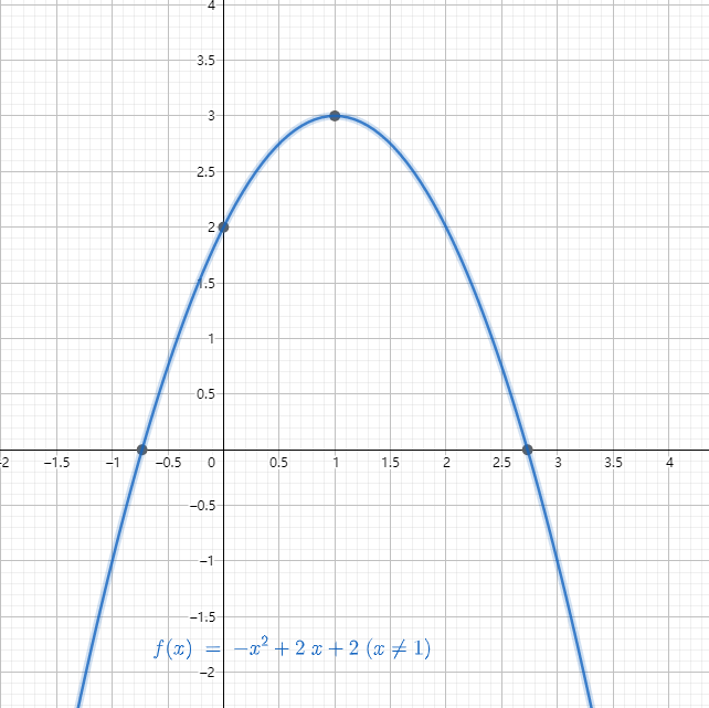
x → 1 x \rightarrow1 x→1时, f ( x ) f(x) f(x)的值如何变化?
我们将这个图像放大了看, x = 1 x=1 x=1附近的点取值非常接近 3 3 3,即当 x x x趋近与 1 1 1时, f ( x ) f(x) f(x)趋近于 3 3 3,用公式表示为
lim x → 1 f ( x ) = 3 \displaystyle\lim _{x \rightarrow 1} f(x)=3 x→1limf(x)=3

注意到在定义域中 x x x取不到 1 1 1这个点,也就是 x = 1 x=1 x=1这个点函数值不存在,但是极限值存在,某一点的极限值只和这一点附近的函数值有关,和这一点本身的取值无关,这个附近的范围称为邻域。
邻域
邻域到底是多大一个范围呢?结合实例来说明一下。
-
美国屡次进犯我国南海,假设有一次美军军舰抵近我国岛屿20海里,我军可能会呼叫对方
You have approached the adjacent waters of China's territorial waters, which seriously threaten China's national security. Please leave immediately.你们已经接近中国领海的邻近水域,这严重威胁到中国的国家安全。请立即离开。根据《联合国海洋法公约》领海宽度为12海里,20海里和12海里虽然差了8海里(约16公里),但在国防安全上毫无疑问是非常邻近的区域。 -
如果小明的爷爷在小明放学的时候给小明打电话“孙子,我在校门口附近等你,你出来就能看到我。”那么这个附近的位置离校门口的距离通常不会超过20米。
现实中讨论的邻近区域的范围会因为具体问题的不同而表现出较大差异。
数学是一种抽象的工具,南海的岛屿和小明学校的校门都可以看做坐标上的点,邻近海域和校门口的邻近位置都在相应点的邻近区域。那么在坐标轴这样的抽象模型中,邻域就是坐标上某点的邻近区域,定义中并不限定具体多远的距离算邻域。一方面现实中的附近千差万别,另一方面定义附近就像定义多少粒沙子才能算一堆沙子一样困难。
当然如果在某些问题中必须限定邻域的范围可以用某些限定词来表述描述,比如去心领域,邻域半径,单侧领域等等。
邻域是一个特殊的区间,以点 a a a为中心点任何开区间称为点 a a a的邻域,记作 U ( a ) U(a) U(a)。
点 a a a的 δ δ δ(英文发音
delta)邻域:设 δ δ δ是一个正数,则开区间(a-δ,a+δ)称为点 a a a的 δ δ δ邻域,记作
U ( a , δ ) = { x ∣ a − δ < x < a + δ } U(a, \delta)=\{x \mid a-\delta
点a称为这个邻域的中心,δ称为这个邻域的半径。由于 a − δ < x < a + δ a-\delta
自变量趋于无穷大时函数的极限
这里分三种情况:
- 自变量趋于正无穷大
- 自变量趋于负无穷大
- 自变量趋于无穷大
定义1(自变量趋于正无穷大)
若对于任意给定的正数 ε \varepsilon ε,存在一个正数 X X X,使得当 x x x 大于 X X X 时,函数 f ( x ) f(x) f(x) 与常数 A A A 之间的差的绝对值小于 ε \varepsilon ε,那么我们称常数 A A A 是当 x x x 趋向正无穷时函数 f ( x ) f(x) f(x) 的极限。
用更简洁的数学语言表示:若 ∀ ε > 0 \forall\varepsilon>0 ∀ε>0, ∃ X > 0 \exists X>0 ∃X>0, 当 x > X x>X x>X 时, 恒有 ∣ f ( x ) − A ∣ < ε |f(x)-A|<\varepsilon ∣f(x)−A∣<ε, 则 lim x → + ∞ f ( x ) = A \displaystyle\lim_{x \rightarrow +\infty} f(x)=A x→+∞limf(x)=A。
示意图如下:
函数自变量趋于正无穷大时的极限定义和数列的极限定义有什么相同点和不同点呢?
相同点是,两个定义中,自变量都是趋向正无穷大,列数的自变量是项数n,项数n趋向无穷就是正无穷,数列项数不可能为负。不同点在于数列极限的定义中的项数n只能为正整数,是离散取值,而函数极限的定义中的自变量x的取值是连续的。
定义2(自变量趋于负无穷大)
若对于任意给定的正数 ε \varepsilon ε,存在一个负数 X X X,使得当 x x x 小于 X X X 时,函数 f ( x ) f(x) f(x) 与常数 A A A 之间的差的绝对值小于 ε \varepsilon ε,那么我们称常数 A A A 是当 x x x 趋向负无穷时函数 f ( x ) f(x) f(x) 的极限。
用更简洁的数学语言表示:若 ∀ ε > 0 \forall\varepsilon>0 ∀ε>0, ∃ X < 0 \exists X<0 ∃X<0, 当 x < X x
x<X 时, 恒有 ∣ f ( x ) − A ∣ < ε |f(x)-A|<\varepsilon ∣f(x)−A∣<ε, 则 lim x → − ∞ f ( x ) = A \displaystyle\lim_{x \rightarrow -\infty} f(x)=A x→−∞limf(x)=A。示意图如下:

定义3(自变量趋于无穷大)
若对于任意给定的正数 ε \varepsilon ε,存在一个正数 X X X,使得当 x x x 的绝对值大于 X X X 时,函数 f ( x ) f(x) f(x) 与常数 A A A 之间的差的绝对值小于 ε \varepsilon ε,那么我们称常数 A A A 是当 x x x 趋向负穷时函数 f ( x ) f(x) f(x) 的极限。
用更简洁的数学语言表示:若 ∀ ε > 0 \forall\varepsilon>0 ∀ε>0, ∃ X > 0 \exists X>0 ∃X>0, 当 ∣ x ∣ > X |x|>X ∣x∣>X 时, 恒有 ∣ f ( x ) − A ∣ < ε |f(x)-A|<\varepsilon ∣f(x)−A∣<ε, 则 lim x → ∞ f ( x ) = A \displaystyle\lim_{x \rightarrow \infty} f(x)=A x→∞limf(x)=A。
注意
-
函数中的 x → ∞ x\rightarrow\infty x→∞是指 ∣ x ∣ → + ∞ |x| \rightarrow+\infty ∣x∣→+∞,而数列极限中的 n → ∞ n\rightarrow\infty n→∞是指 n → + ∞ n\rightarrow+\infty n→+∞;
-
极限 lim x → ∞ f ( x ) \displaystyle\lim_{x \rightarrow \infty}f(x) x→∞limf(x)存在的充要条件是极限 lim x → − ∞ f ( x ) \displaystyle\lim_{x \rightarrow-\infty}f(x) x→−∞limf(x)及 lim x → + ∞ f ( x ) \displaystyle\lim _{x \rightarrow+\infty}f(x) x→+∞limf(x)都存在并且相等。即:
lim x → ∞ f ( x ) = A ⇔ lim x → + ∞ f ( x ) = lim x → − ∞ f ( x ) = A \lim _{x \rightarrow \infty} f(x)=A \Leftrightarrow \lim _{x \rightarrow+\infty} f(x)=\lim _{x \rightarrow-\infty} f(x)=A x→∞limf(x)=A⇔x→+∞limf(x)=x→−∞limf(x)=A
示意图如下:


自变量趋于有限值时函数的极限
定义
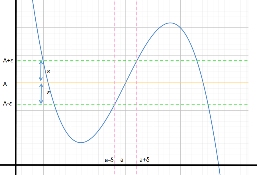
如果对于任意正数 ε,总能找到一个正数 δ,使得当 x x x 落在距离 x 0 x_0 x0 不超过 δ 的范围内(但不等于 x 0 x_0 x0),函数 f ( x ) f(x) f(x) 与常数 A A A 之间的差的绝对值小于 ε,那么我们称常数 A A A 是当 x x x 趋向 x 0 x₀ x0 时函数 f ( x ) f(x) f(x) 的极限。这表示随着 x x x 越来越接近 x 0 x_0 x0,函数 f ( x ) f(x) f(x) 无限接近于常数 A A A。
用更简洁的数学语言表示:若 ∀ ε > 0 \forall\varepsilon>0 ∀ε>0, ∃ δ > 0 \exists\delta>0 ∃δ>0,当 0 < ∣ x − x 0 ∣ < δ 0<\left|x-x_{0}\right|<\delta 0<∣x−x0∣<δ 时, ∣ f ( x ) − A ∣ < ε |f(x)-A|< \varepsilon ∣f(x)−A∣<ε,则 lim x → x 0 f ( x ) = A \displaystyle\lim _{x \rightarrow x_{0}} f(x)=A x→x0limf(x)=A。
示意图如下,图像中的曲线是函数 f ( x ) f ( x ) f(x),图像中的 a a a是定义中的 x 0 x_{0} x0:
注意
-
对于 U ˚ ( x 0 , δ ) \mathring{U}\left(x_{0}, \delta\right) U˚(x0,δ),字母 U U U上面有一个小圆圈,这表示去心邻域,即邻域的范围不包含邻域中心 x 0 x_{0} x0 那一点。
-
函数在某一点的极限的几何意义: 对任意给定的 ε > 0 \varepsilon>0 ε>0 , 总存在 U ˚ ( x 0 , δ ) \mathring{U}\left(x_{0}, \delta\right) U˚(x0,δ), 当 f ( x ) ∈ U ( A , ε ) f(x) \in {U}\left(A, \varepsilon\right) f(x)∈U(A,ε) 时, x ∈ U ˚ ( x 0 , δ ) x \in \mathring{U}\left(x_{0}, \delta\right) x∈U˚(x0,δ) 。
-
ε \varepsilon ε是用来刻画 f ( x ) f(x) f(x)与 A A A的接近程度,指 f ( x ) f(x) f(x)与 A A A无限靠近, δ \delta δ 是用来刻画 x → x 0 x \rightarrow x_{0} x→x0 这个接近过程, δ \delta δ 总是存在意味着在 x x x 向 x 0 x_0 x0 的过程中,即 U ˚ ( x 0 , δ ) \mathring{U}\left(x_{0}, \delta\right) U˚(x0,δ) 范围内, x x x 处处有定义。
-
研究函数在某一点的极限是看这一点的邻域的取值,和这一点本身的取值无关。
具体来说: lim x → x 0 f ( x ) \displaystyle\lim _{x \rightarrow x_{0}} f(x) x→x0limf(x)是否存在,极限值等于多少与 f ( x ) f(x) f(x)在 x = x 0 x=x_{0} x=x0处有没有定义无关。如果 x 0 x_{0} x0 处有定义, x 0 x_{0} x0 处的函数值等于多少也与极限值无关。极限值只与 x = x 0 x=x_{0} x=x0 的去心邻域 U ˚ ( x 0 , δ ) \mathring{U}\left(x_{0}, \delta\right) U˚(x0,δ) 函数值有关,要使 lim x → x 0 f ( x ) \displaystyle\lim _{x \rightarrow x_{0}} f(x) x→x0limf(x)存在, f ( x ) f(x) f(x)必须在 x = x 0 x=x_{0} x=x0的某去心邻域 U ˚ ( x 0 , δ ) \mathring{U}\left(x_{0}, \delta\right) U˚(x0,δ)处处有定义。
函数极限的基本运算
同数列极限一样,函数极限也有相应的基本运算法则。这些法则适用于多项式函数、三角函数、对数函数、指数函数等等各种函数。这里仅给出公式,对于每种函数求极限的例题和练习在后面的章节。
如果 L L L, M M M, x 0 x_0 x0 和 k k k 都是实数,且 lim f ( x ) = L \displaystyle\lim f(x)=L limf(x)=L 和 lim g ( x ) = M \displaystyle\lim g(x)=M limg(x)=M ,那么无论 x → x 0 x \rightarrow x_0 x→x0 还是 x → ∞ x \rightarrow \infty x→∞ 都有:
- 和法则:两个函数之和的极限等于它们的极限之和。
lim ( f ( x ) + g ( x ) ) = L + M \displaystyle\lim (f(x)+g(x))=L+M lim(f(x)+g(x))=L+M
- 差法则 :两个函数之差的极限等于它们的极限之差。
lim ( f ( x ) − g ( x ) ) = L − M \displaystyle\lim (f(x)-g(x))=L-M lim(f(x)−g(x))=L−M
- 积法则 :两个函数之积的极限等于它们的极限之积。
lim ( f ( x ) ⋅ g ( x ) ) = L ⋅ M \displaystyle\lim (f(x) \cdot g(x))=L \cdot M lim(f(x)⋅g(x))=L⋅M
- 乘常数法则:常数乘一个函数后的极限等于该常数乘该函数的极限。
lim ( k ⋅ f ( x ) ) = k ⋅ L \displaystyle\lim (k \cdot f(x))=k \cdot L lim(k⋅f(x))=k⋅L
- 商法则:两个函数之商的极限等于它们的极限之商,如果分母的极限不为零。
lim f ( x ) g ( x ) = L M , M ≠ 0 \displaystyle\lim \frac{f(x)}{g(x)}=\frac{L}{M}, \quad M \neq 0 limg(x)f(x)=ML,M=0
- 冪法则:如果 r r r 和 s s s 都是整数, s ≠ 0 s \neq 0 s=0 , 那么只要 L r s L^{\frac{r}{s}} Lsr 是实数,函数的有理幂的极限等于该函数极限的同样的幂,如果后者是实数。
lim ( f ( x ) ) r s = L r s \displaystyle\lim (f(x))^{\frac{r}{s}}=L^{\frac{r}{s}} lim(f(x))sr=Lsr
1.1.3 左极限和右极限
引言
想象一下在中印交界的位置,有一个地方是垂直的喜马拉雅山崖。

阿三从山崖的左边疯狂地想要突破山崖爬过来,但是无论多么疯狂的举动他们也不能突破,只能从左边无限靠近山崖的底端,那么山崖的底端就是阿三从左边过来的极限位置。
山崖上插着祖国的红旗,我们的守军从右边防御敌人也只能从右边无限靠近红红旗的位置。

如果建立一个坐标轴,阿三水平位置从左边无限接近 x 0 x_{0} x0的时候,横坐标都比 x 0 x_{0} x0更小,所以用 x → x 0 − x\rightarrow x_{0}^{-} x→x0− 来描述横坐标 x x x 趋近 x 0 x_{0} x0 但小于 x 0 x_{0} x0 的状态。横坐标 x → x 0 − x\rightarrow x_{0}^{-} x→x0− 时他们的纵坐标 f ( x ) f(x) f(x) 会越来越接近 y 1 y1 y1 ,即 f ( x ) f(x) f(x) 在 x = x 0 x=x_0 x=x0 的左极限为 y 1 y1 y1 ,记为: lim x → x 0 − f ( x ) = y 1 \displaystyle\lim_{x \rightarrow x_{0}^{-}}{f\left( x \right)}=y_{1} x→x0−limf(x)=y1。
我们的守军从右边过来,我们的水平位置无限接近 x 0 x_{0} x0 的时候,高度会越来越接近 y 2 y2 y2 ,因为从右边过来的横坐标都比 x 0 x_{0} x0 更大,所以用 x → x 0 + x\rightarrow x_{0}^{+} x→x0+来描述横坐标 x x x 趋近 x 0 x_{0} x0 但大于 x 0 x_{0} x0 的状态。横坐标 x → x 0 + x\rightarrow x_{0}^{+} x→x0+时我们的高度 f ( x ) f(x) f(x) 会越来越接近 y 2 y2 y2 ,即 f ( x ) f(x) f(x) 在 x = x 0 x=x0 x=x0 的右极限为 y 2 y2 y2 ,数学表达式 lim x → x 0 + f ( x ) = y 2 \displaystyle\lim_{x \rightarrow x_{0}^{+}}{f\left( x \right)}=y_{2} x→x0+limf(x)=y2。
如果在 x 0 x_{0} x0 的后面不加正负号,那么 lim x → x 0 f ( x ) = y \displaystyle\lim_{x \rightarrow x_{0}^{}}{f\left( x \right)}=y_{} x→x0limf(x)=y表示双侧极限,当且仅当左右极限同时存在且相等时双侧极限才存在。
定义
左极限
若对任意给定的 ε > 0 \varepsilon>0 ε>0, 总存在 δ > 0 \delta>0 δ>0, 当 x 0 − δ < x < x 0 x_{0}-\delta
右极限
若对任意给定的 ε > 0 \varepsilon>0 ε>0, 总存在 δ > 0 \delta>0 δ>0, 当 x 0 < x < x 0 + δ x_{0}
lim x → x 0 + f ( x ) = A \displaystyle\lim _{x \rightarrow x_{0}^{+}} f(x)=A x→x0+limf(x)=A, 或 f ( x 0 + ) = A f\left(x_{0}^{+}\right)=A f(x0+)=A ,或 f ( x 0 + 0 ) = A f\left(x_{0}+0\right)=A f(x0+0)=A
需要分左、右极限求极限的常见问题
- 分段函数在分界点处的极限, 而在该分界点两侧函数表达式不同(这里也包括带有 绝对值的函数, 如 lim x → 0 ∣ x ∣ x \displaystyle\lim _{x \rightarrow 0} \frac{|x|}{x} x→0limx∣x∣ );

-
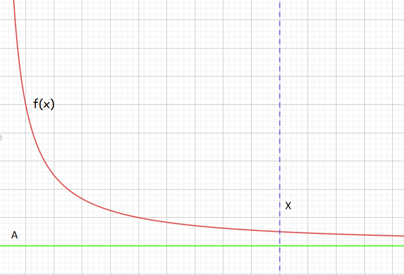
e ∞ \mathrm{e}^{\infty} e∞型极限 (如 lim x → 0 e 1 x \displaystyle\lim _{x \rightarrow 0} \mathrm{e}^{\frac{1}{x}} x→0limex1, lim x → ∞ e x \displaystyle\lim _{x \rightarrow \infty} \mathrm{e}^{x} x→∞limex, lim x → ∞ e − x \displaystyle\lim_{x \rightarrow \infty} \mathrm{e}^{-x} x→∞lime−x)
下图为 e 1 x e^{\frac{1}{x}} ex1 示意图,左极限 lim x → 0 − e 1 x = 0 \displaystyle\lim _{x \rightarrow 0^{-}} \mathrm{e}^{\frac{1}{x}}=0 x→0−limex1=0,右极限 lim x → 0 + e 1 x = + ∞ \displaystyle\lim _{x \rightarrow 0^{+}} \mathrm{e}^{\frac{1}{x}}=+\infty x→0+limex1=+∞,右极限不存在,所以 lim x → 0 e 1 x \displaystyle\lim _{x \rightarrow 0} \mathrm{e}^{\frac{1}{x}} x→0limex1 不存在。

下图为 e x e^x ex 的示意图,左极限 lim x → − ∞ e x = 0 \displaystyle\lim _{x \rightarrow-\infty} \mathrm{e}^{x}=0 x→−∞limex=0,右极限 lim x → + ∞ e x = + ∞ \displaystyle\lim _{x \rightarrow+\infty} \mathrm{e}^{x}=+\infty x→+∞limex=+∞,右极限不存在,则 lim x → ∞ e x \displaystyle\lim _{x \rightarrow \infty} \mathrm{e}^{x} x→∞limex 不存在。
注意 e ∞ ≠ ∞ , e + ∞ = + ∞ , e − ∞ = 0 \mathrm{e}^{\infty} \neq \infty, \mathrm{e}^{+\infty}=+\infty,\mathrm{e}^{-\infty}=0 e∞=∞,e+∞=+∞,e−∞=0.

- arctan ∞ \arctan \infty arctan∞ 型极限 (如 lim x → 0 a r c t a n 1 x \displaystyle\lim_{x \rightarrow 0}{arctan} \frac{1}{x} x→0limarctanx1, lim x → ∞ a r c t a n x \displaystyle\lim _{x \rightarrow \infty}{arctan} x x→∞limarctanx)
lim x → − ∞ arctan x = − π 2 \displaystyle\lim _{x \rightarrow-\infty} \arctan x=-\frac{\pi}{2} x→−∞limarctanx=−2π, lim x → + ∞ arctan x = π 2 \displaystyle\lim _{x \rightarrow+\infty} \arctan x=\frac{\pi}{2} x→+∞limarctanx=2π,左右极限都存在但是不相等,所以 lim x → ∞ arctan x \displaystyle\lim _{x\rightarrow \infty}\arctan x x→∞limarctanx不存在。
lim x → 0 − arctan 1 x = − π 2 \displaystyle\lim _{x\rightarrow 0^{-}}\arctan\frac{1}{x}=-\frac{\pi}{2} x→0−limarctanx1=−2π, lim x → 0 + arctan 1 x = π 2 \displaystyle\lim _{x \rightarrow 0^{+}}\arctan\frac{1}{x}=\frac{\pi}{2} x→0+limarctanx1=2π,左右极限都存在但是不相等,所以 lim x → 0 arctan 1 x \displaystyle\lim_{x\rightarrow 0}\arctan\frac{1}{x} x→0limarctanx1 不存在。
【注意】
arctan ∞ ≠ π 2 \arctan \infty \neq \frac{\pi}{2} arctan∞=2π, arctan ( + ∞ ) = π 2 \arctan (+\infty)=\frac{\pi}{2} arctan(+∞)=2π, arctan ( − ∞ ) = − π 2 \arctan (-\infty)=-\frac{\pi}{2} arctan(−∞)=−2π.下图为 arctan x \arctan x arctanx 示意图

1.1.4定理:极限存在的充要条件
极限 lim x → x 0 f ( x ) \displaystyle\lim _{x \rightarrow x_{0}} f(x) x→x0limf(x) 存在的充要条件是左极限 lim x → x 0 − f ( x ) \displaystyle\lim _{x \rightarrow x_{0}^{-}} f(x) x→x0−limf(x) 及右极限 lim x → x 0 + f ( x ) \displaystyle\lim _{x \rightarrow x_{0}^{+}} f(x) x→x0+limf(x)存在并且相等.
lim x → x 0 f ( x ) = A ⇔ lim x → + x 0 f ( x ) = lim x → − x 0 f ( x ) = A \lim _{x \rightarrow x_0} f(x)=A \Leftrightarrow \lim _{x \rightarrow+x_0} f(x)=\lim _{x \rightarrow-x_0} f(x)=A x→x0limf(x)=A⇔x→+x0limf(x)=x→−x0limf(x)=A1.1.5极限不存在的常见情况
通过极限存在的充要条件,可以归纳常见的极限不存在的情况,以下示例暂且了解,在学习了各种函数的。
自变量趋于某一个值时函数值趋于无穷
自变量趋于某一个值时函数值趋于无穷,则函数在这一点极限值不存在。
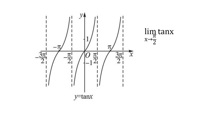
比如正切函数在自变量 x → π 2 \displaystyle x\rightarrow \frac{\pi}{2} x→2π 时函数值趋于无穷,所以正切函数在 π 2 \displaystyle\frac{\pi}{2} 2π 的极限值不存在。
函数在自变量的某点只存在左极限或者只存在右极限
函数在自变量的某点只存在左极限或者只存在右极限,则函数在自变量的这一点极限值不存在。
比如 e − 1 x \displaystyle e^{-\frac1x} e−x1 在 x → 0 \displaystyle x\rightarrow 0 x→0 时只存在右极限不存在左极限。

函数自变量某点虽然左右极限都存在但左右极限不相等
函数自变量某点虽然左右极限都存在但左右极限不相等,则函数在自变量的这一点极限值不存在。
比如符号函数在 x x x 趋于 0 0 0 时左右极限都存在但不相等。

函数自变量x趋于某一点时函数值震荡
函数自变量 x x x 趋于某一点时函数值震荡,则函数在自变量的这一点极限值不存在。
比如 sin 1 x \displaystyle\sin\frac1x sinx1在 x x x 趋于 0 0 0时函数值振荡。

自变量 x x x 某点的任意无穷小邻域内有无定义点
自变量x某点的任意无穷小邻域内有无定义点,则函数在自变量的这一点极限值不存在。
比如函数 f ( x ) = s i n ( x s i n 1 x ) ( x s i n 1 x ) \displaystyle f(x)=\frac{sin(xsin{\frac{1}{x}})}{(xsin\frac{1}{x})} f(x)=(xsinx1)sin(xsinx1) 在 x x x 等于 1 k π \frac1{kπ} kπ1 ( K K K为整数)时分母为零,为无定义点,所以此函数在 x x x 趋于 0 0 0 时极限不存在。
-
相关阅读:
kubernetes配置资源管理
uLua:在AVR 8位微控制器上运行的高效Lua编译器与迭代器详细指南
DC/DC开关电源学习笔记(六)开关电源电路集成及封装工艺
超实用!了解github的热门趋势和star排行是必须得!
【MySQL】-【变量、流程控制、游标】
Python语言程序设计 习题3
MapReduce Partition 分区
send line/selection to terminal
DDD领域驱动设计总结和C#代码示例
MyBatis-Plus配置
- 原文地址:https://blog.csdn.net/weixin_40171190/article/details/127896680