【毕业设计】大数据客户价值分析（RFM模型）

---

1 简介

🔥 Hi，大家好，这里是丹成学长的毕设系列文章！

🔥 对毕设有任何疑问都可以问学长哦!

这两年开始，各个学校对毕设的要求越来越高，难度也越来越大… 毕业设计耗费时间，耗费精力，甚至有些题目即使是专业的老师或者硕士生也需要很长时间，所以一旦发现问题，一定要提前准备，避免到后面措手不及，草草了事。

为了大家能够顺利以及最少的精力通过毕设，学长分享优质毕业设计项目，今天要分享的新项目是

🚩 大数据分析：客户价值分析 RFM模型

🥇学长这里给一个题目综合评分(每项满分5分)

• 难度系数：4分
• 工作量：4分
• 创新点：3分

🧿 选题指导, 项目分享：

https://gitee.com/yaa-dc/BJH/blob/master/gg/cc/README.md

2 数据预处理

# 加载必要的库
import pandas as pd
import numpy as np
from pandas import DataFrame,Series
import seaborn as sns
import matplotlib.pyplot as plt
plt.style.use('fivethirtyeight')
%matplotlib inline
from warnings import filterwarnings
filterwarnings('ignore') 
import os
import datetime

import plotly.offline as py
from plotly.offline import init_notebook_mode,iplot
import plotly.graph_objs as go
from plotly import tools
init_notebook_mode(connected=True)
import plotly.figure_factory as ff

from sklearn.cluster import MiniBatchKMeans, KMeans
from sklearn.metrics.pairwise import pairwise_distances_argmin
from sklearn.datasets import make_blobs
# 导入数据
path='/home/kesci/input/7947606275/data.csv'
df=pd.read_csv(path,dtype={'CustomerID':str,'InvoiceID':str})
df.head()
1
2
3
4
5
6
7
8
9
10
11
12
13
14
15
16
17
18
19
20
21
22
23
24
25
26
27

数据去重与异常数据处理

df=df.drop_duplicates()
# 查看描述统计
df.describe()
df.loc[df['UnitPrice']<0].UnitPrice.count()
# 查看这2行的Description是什么
df.loc[df['UnitPrice']<0,['UnitPrice','Description']]
# 删除UnitPrice小于0的和Quantity小于0的数据
df=df[(df['UnitPrice']>=0) & (df['Quantity']>0)]

1
2
3
4
5
6
7
8
9

3 数据分析

3.1 数据准备

# 减少重复数据
df_f = df
df_f.drop_duplicates(subset=['InvoiceNo', 'CustomerID'], keep="first", inplace=True)
#计算购买频率
frequency_df = df_f.groupby(by=['CustomerID'], as_index=False)['InvoiceNo'].count()
frequency_df.columns = ['CustomerID','Frequency']
frequency_df.set_index('CustomerID',drop=True,inplace=True)
frequency_df.head()
1
2
3
4
5
6
7
8

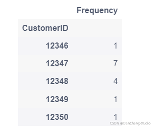
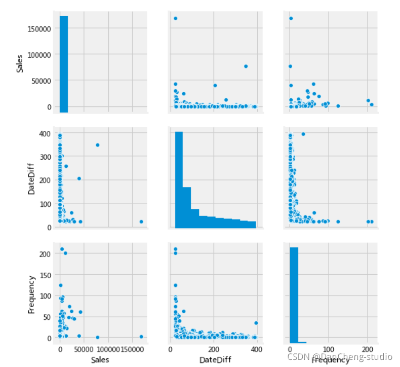
3.2 数据可视化

3.2.1 查看数据大概分布

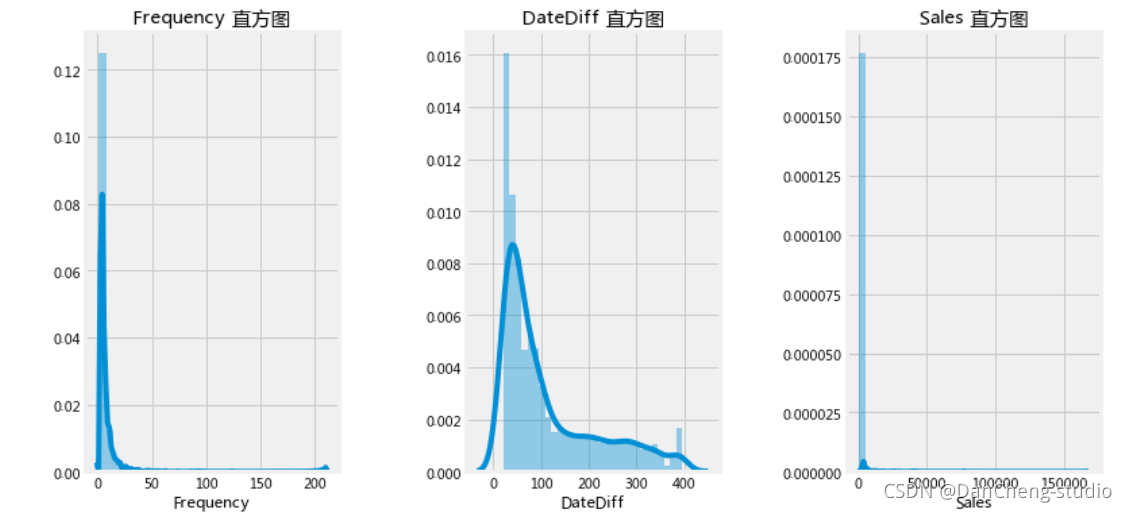
3.2.2 分布直方图

plt.figure(1,figsize=(12,6))
n=0
for x in ['Frequency','DateDiff','Sales']:
    n+=1
    plt.subplot(1,3,n)
    plt.subplots_adjust(hspace=0.5,wspace=0.5)
    sns.distplot(df_rfm[x],bins=30)
    plt.title('{} 直方图'.format(x))
plt.show()
1
2
3
4
5
6
7
8
9

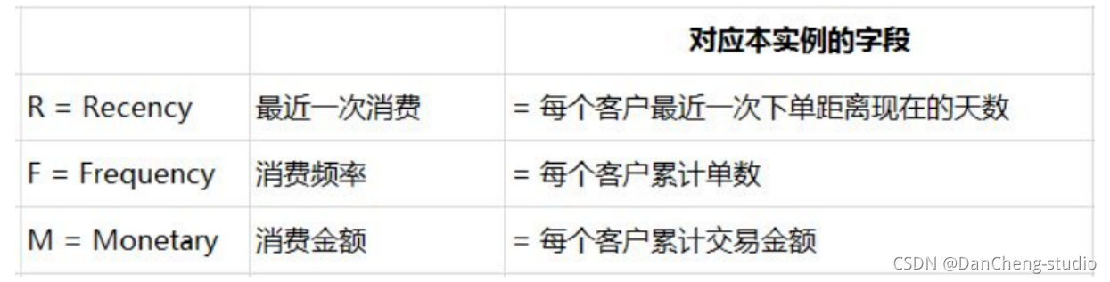
4 R、F、M模型

4.1 模型含义

4.2 R、F、M的均值

计算用于划分客户的阙值，R、F、M的均值（*通过分布直方图可以发现该份数据不适合用中位数来分层，因此这里用均值做分层）

rmd = df_rfm['DateDiff'].mean()
fmd = df_rfm['Frequency'].mean()
mmd = df_rfm['Sales'].mean()
rmd,fmd,mmd
def customer_type(frame): 
    customer_type = []
    for i in range(len(frame)):
        if frame.iloc[i,1]<=rmd and frame.iloc[i,2]>=fmd and frame.iloc[i,0]>=mmd:
            customer_type.append('重要价值用户')
        elif  frame.iloc[i,1]>rmd and frame.iloc[i,2]>=fmd and frame.iloc[i,0]>=mmd:
            customer_type.append('重要唤回用户')
        elif  frame.iloc[i,1]<=rmd and frame.iloc[i,2]<fmd and frame.iloc[i,0]>=mmd:
            customer_type.append('重要深耕用户')
        elif  frame.iloc[i,1]>rmd and frame.iloc[i,2]<fmd and frame.iloc[i,0]>=mmd:
            customer_type.append('重要挽留用户')
        elif  frame.iloc[i,1]<=rmd and frame.iloc[i,2]>=fmd and frame.iloc[i,0]<mmd:
            customer_type.append('潜力用户')
        elif  frame.iloc[i,1]>rmd and frame.iloc[i,2]>=fmd and frame.iloc[i,0]<mmd:
            customer_type.append('一般维持用户')
        elif  frame.iloc[i,1]<=rmd and frame.iloc[i,2]<fmd and frame.iloc[i,0]<mmd:
            customer_type.append('新用户')
        elif frame.iloc[i,1]>rmd and frame.iloc[i,2]<fmd and frame.iloc[i,0]<mmd:
            customer_type.append('流失用户')
    frame['classification'] = customer_type
    customer_type(df_rfm)

print('不同类型的客户总数：')
print('--------------------')
df_rfm.groupby(by='classification').size().reset_index(name='客户数')
1
2
3
4
5
6
7
8
9
10
11
12
13
14
15
16
17
18
19
20
21
22
23
24
25
26
27
28
29

4.3 不同类型的客户消费份额

4.4 利用最近交易间隔，交易金额进行细分

假设不规定8个分类利用模型来选择最优分类，利用最近交易间隔，交易金额进行细分

X= df_rfm[['Sales' , 'DateDiff' ,'Frequency']].iloc[: , :].values
inertia = []
for n in range(1 , 11):
    algorithm = (KMeans(n_clusters = n ,init='k-means++', n_init = 10 ,max_iter=300, 
                        tol=0.0001,  random_state= 111  , algorithm='elkan') )
    algorithm.fit(X)
    inertia.append(algorithm.inertia_)
 algorithm = (KMeans(n_clusters = 5,init='k-means++', n_init = 10 ,max_iter=300, 
                        tol=0.0001,  random_state= 111  , algorithm='elkan') )
algorithm.fit(X)
labels3 = algorithm.labels_
centroids3 = algorithm.cluster_centers_
df_rfm['label3'] =  labels3
trace1 = go.Scatter3d(
    x= df_rfm['Sales'],
    y= df_rfm['DateDiff'],
    z= df_rfm['Frequency'],
    mode='markers',
     marker=dict(
        color = df_rfm['label3'], 
        size=10,
        line=dict(
            color= df_rfm['label3'],
#             width= 10
        ),
        opacity=0.8
     )
)
data = [trace1]
layout = go.Layout(
#     margin=dict(
#         l=0,
#         r=0,
#         b=0,
#         t=0
#     )
    height=800,
    width=800,
    title= 'Sales  VS  DateDiff  VS  Frequency',
    scene = dict(
            xaxis = dict(title  = 'Sales'),
            yaxis = dict(title  = 'DateDiff'),
            zaxis = dict(title  = 'Frequency')
        )
)
fig = go.Figure(data=data, layout=layout)
py.offline.iplot(fig)
1
2
3
4
5
6
7
8
9
10
11
12
13
14
15
16
17
18
19
20
21
22
23
24
25
26
27
28
29
30
31
32
33
34
35
36
37
38
39
40
41
42
43
44
45
46
47

5 最后