Pandas基础入门知识点总结

目录

1、pandas 常用类

1.1 Series

1.1.1创建 Series

1.1.2 访问 Series 数据

1.1.3 更新、插入和删除

1.2 DataFrame

1.2.1 创建 DataFrame

1.2.2 访问DataFrame首尾数据

1.2.3 更新、插入和删除（列操作）

1.3 Index

1.3.1 创建 Index

1.3.2 常用方法

2、DataFrame 基础操作

2.1 索引

2.1.1 基础化索引

2.1.2 loc 方法和 iloc方法（行、列操作）

2.1.3 行追加append

2.1.4 删除数据行

2.1.5 MultiIndex

2.2 排序

2.2.1 sort_index 方法

2.2.2 sort_values 方法

2.3 合并

2.3.1 堆叠合并

3、时间数据

3.1 Python 模块time

3.1.1 time模块

3.1.2 datetime 模块

3.1.3 timedelta 类，时间加减

3.2 Pandas 时间 Timedelta

3.3 Pandas 时间转化 to_datetime

3.4  Pandas 时间序列 date_range        

---

1、pandas 常用类

1.1 Series

        Series 由一组数据以及一组与之对应的数据标签（即索引）组成。Series 对象可以视作一个NumPy 的 ndarray ，因此许多NumPy库函数可以作用于 series。

1.1.1创建 Series

        Pandas Series 类似表格中的一个列（column），类似于一维数组，可以保存任何数据类型，本质上是一个 ndarray。Series 由索引（index）和列组成，函数如下：

pandas.Series( data=None, index=None, dtype=None, name=None, copy=False)

参数说明：

• data：一组数据(ndarray 类型)。

• index：数据索引标签，如果不指定，默认从 0 开始。

• dtype：数据类型，默认会自己判断。

• name：设置该 Series 名称。

• copy：拷贝数据，默认为 False。仅影响 Series 和 ndarray 数组

通过 ndarray 创建 Series

import numpy as np
import pandas as pd
print('通过 ndarray 创建的 Series 为：\n', pd.Series(np.arange(5), index=['a', 'b', 'c', 'd', 'e'], name='ndarray'))

运行结果：

通过 ndarray 创建的 Series 为：
 a    0
b    1
c    2
d    3
e    4
Name: ndarray, dtype: int32

        若数据存放在 dict 中，则可以通过 dict 创建 Series，此时 dict 的键名（key）作为 Series 的索引，其值会作为 Series 的值，因此无需传入 index 参数。通过dict创建 Series 对象，代码如下：

通过 dict 创建 Series

import numpy as np
import pandas as pd
dit = {'a': 0, 'b': 1, 'c': 2, 'd': 3}
print('通过 dict 创建的 Series 为：\n', pd.Series(dit))

运行结果：

通过 dict 创建的 Series 为：
 a    0
b    1
c    2
d    3
dtype: int64

通过 list 创建 Series

import numpy as np
import pandas as pd
list1 = [1, 2, 3, 4, 5]
list2 = [10, 2, 36, 4, 25]
print('通过 list 创建的 Series 为：\n', pd.Series(list1))  # 索引为默认
print('通过 list 创建的 Series 为：\n', pd.Series(list2, index=['a', 'b', 'c', 'd', 'e'], name='list'))

运行结果：

通过 list 创建的 Series 为：
 0    1
1    2
2    3
3    4
4    5
dtype: int64
通过 list 创建的 Series 为：
 a    10
b     2
c    36
d     4
e    25
Name: list, dtype: int64

---

import numpy as np
import pandas as pd
list1 = [1, 2, 3, 4, 5]
series = pd.Series(list1, index=['a', 'b', 'c', 'd', 'e'], name='list')
print('通过 dict 创建的 Series 为：\n', series)
print('数组形式返回 Series 为：', series.values)
print('Series 的 Index 为：', series.index)
print('Series 的 形状为：', series.shape)
print('Series 的 维度为：', series.ndim)
print('Series 对象的个数为：', series.size)
print('返回 Series 索引列表为：', series.axes)

运行结果：

通过 dict 创建的 Series 为：
 a    1
b    2
c    3
d    4
e    5
Name: list, dtype: int64
数组形式返回 Series 为： [1 2 3 4 5]
Series 的 Index 为： Index(['a', 'b', 'c', 'd', 'e'], dtype='object')
Series 的 形状为： (5,)
Series 的 维度为： 1
Series 对象的个数为： 5
返回 Series 索引列表为： [Index(['a', 'b', 'c', 'd', 'e'], dtype='object')]

1.1.2 访问 Series 数据

        索引和切片是 Series 最常用的操作之一，通过索引位置访问 Series 的数据与 ndarray 相同。Series 使用标签切片时，其末端时包含的，使用位置数值切片，其末端是不包含的。 

import numpy as np
import pandas as pd
# 创建 Series
s1 = pd.Series(np.arange(1, 6))
print('通过 ndarray 创建的 Series 为：\n', s1)  # 索引为默认
print(f"s1.index为：\n{s1.index}")
print(f"s1.index强制转换为列表输出为：\n{list(s1.index)}")
# 通过标签取得对应的值，或进行修改
s1[2] = 100
# print(s1[-1])   # 无法通过反向索引
s1[-1] = 99     # 新增一行数据
print(f"现在的Series为：\n{s1}")
print(f"s1[-1]:  {s1[-1]}")   # 标签中存在-1

运行结果：

通过 ndarray 创建的 Series 为：
 0    1
1    2
2    3
3    4
4    5
dtype: int32
s1.index为：
RangeIndex(start=0, stop=5, step=1)
s1.index强制转换为列表输出为：
[0, 1, 2, 3, 4]
现在的Series为：
 0      1
 1      2
 2    100
 3      4
 4      5
-1     99
dtype: int64
s1[-1]:  99

---

import numpy as np
import pandas as pd
dit = {'a': 0, 'b': 1, 'c': 2, 'd': 3}
print('通过 dict 创建的 Series 为：\n', pd.Series(dit))
# 通过标签取得相应的值，或进行修改
dit['s'] = 9
print(f"dit['b'] = {dit['b']}")

运行结果：

通过 dict 创建的 Series 为：
 a    0
b    1
c    2
d    3
dtype: int64
dit['b'] = 1

---

import numpy as np
import pandas as pd
list1 = [1, 2, 3, 4, 5]
series = pd.Series(list1, index=['a', 'b', 'c', 'd', 'e'], name='list')
print('通过 dict 创建的 Series 为：\n', series)
print(f"Series 位于第 1 位置的数据为：{series[0]}")
# 通过索引名称（标签）也可以访问Series 数据
print(f"Series中 Index 为 ‘b’的数据为：{series['b']}")
print(f"bool 类型的 Series 为：\n{series < 4}")
print(f"通过bool 数组访问Series 为：\n{series[series < 4]}")

运行结果：

通过 dict 创建的 Series 为：
 a    1
b    2
c    3
d    4
e    5
Name: list, dtype: int64
Series 位于第 1 位置的数据为：1
Series中 Index 为 ‘b’的数据为：2
bool 类型的 Series 为：
a     True
b     True
c     True
d    False
e    False
Name: list, dtype: bool
通过bool 数组访问Series 为：
a    1
b    2
c    3
Name: list, dtype: int64

1.1.3 更新、插入和删除

import numpy as np
import pandas as pd
list1 = [1, 2, 3, 4, 5]
series = pd.Series(list1, index=['a', 'b', 'c', 'd', 'e'], name='list')
print('通过 dict 创建的 Series 为：\n', series)
# 更新元素
series['b'] = 9
print(f"更新后的 Series 为：\n{series}")
# 在原 Series 上插入（追加）新的Series
series1 = pd.Series([4, 5], index=['f', 'g'])
# 追加
print(f"在 series 后插入 series1，结果为：\n{series.append(series1)}")
# 添加单个元素
series1['h'] = 7
print(f"插入单个数据后 series1：\n{series1}")
# 删除 Series 元素
series.drop('e', inplace=True)
print('删除索引 e 对应的数据后的 series 为：\n', series)

 运行结果：

通过 dict 创建的 Series 为：
 a    1
b    2
c    3
d    4
e    5
Name: list, dtype: int64
更新后的 Series 为：
a    1
b    9
c    3
d    4
e    5
Name: list, dtype: int64
在 series 后插入 series1，结果为：
a    1
b    9
c    3
d    4
e    5
f    4
g    5
dtype: int64
插入单个数据后 series1：
f    4
g    5
h    7
dtype: int64
删除索引 e 对应的数据后的 series 为：
 a    1
b    9
c    3
d    4
Name: list, dtype: int64

1.2 DataFrame

        DataFrame 是 pandas 基本数据结构，类似于数据库中的表。 DataFrame 既有行索引，也有列索引，它可以看作 Series 组成的 dict ，每个 Series 看作 DataFrame 的一个列。

1.2.1 创建 DataFrame

        DataFrame 函数用于创建 DataFrame 对象，其基本语法格式如下：

class pandas.DataFrame(data, index, columns, dtype, copy) 

        创建 DataFrame 的方法由很多，常见的一种是传入一个由等长 list 或 ndarray 组成的 dict。

若没有传入 columns 参数，则传入的 dict 的键会被当做列名。

 使用字典创建 DataFrame 对象

import numpy as np
import pandas as pd
# 通过 dict 创建 DataFrame
dict1 = {'col1': [0, 1, 2, 3, 4], 'col2': [5, 6, 7, 8, 9]}
print(f"痛过 dict 创建的 DataFrame 为：\n{pd.DataFrame(dict1,index=['a', 'b', 'c', 'd', 'e'])}")
# 通过 list 创建 DataFrame
list2 = [[0, 5, 1], [1, 6, 5], [2, 6, 3], [8, 9, 5], [8, 3, 4]]
print(f"痛过 list 创建的 DataFrame 为：\n{pd.DataFrame(list2,index=['a', 'b', 'c', 'd', 'e'], columns=['col1', 'col2', 'col3'])}")

运行结果：

痛过 dict 创建的 DataFrame 为：
   col1  col2
a     0     5
b     1     6
c     2     7
d     3     8
e     4     9
痛过 list 创建的 DataFrame 为：
   col1  col2  col3
a     0     5     1
b     1     6     5
c     2     6     3
d     8     9     5
e     8     3     4

使用嵌套列表创建：

import numpy as np
import pandas as pd
data = [['xiaoming', 20], ['lina', 35], ['jam', 24]]
# 未分配列标签
df = pd.DataFrame(data)
print('使用嵌套列表创建的 DataFrame(未分配列标签) 为：\n', df)
# 分配列标签
df1 = pd.DataFrame(data, columns=['name', 'Age'])
print('使用嵌套列表创建的 DataFrame(分配列标签) 为：\n', df1)

运行结果：

使用嵌套列表创建的 DataFrame(未分配列标签) 为：
           0   1
0  xiaoming  20
1      lina  35
2       jam  24
使用嵌套列表创建的 DataFrame(分配列标签) 为：
        name  Age
0  xiaoming   20
1      lina   35
2       jam   24

 使用列表嵌套字典创建 DataFrame 对象

import numpy as np
import pandas as pd
data = [{'a': 1, 'b': 2}, {'a': 5, 'b': 10, 'c': 20}]
df = pd.DataFrame(data, index=['first', 'second'])
# 如果其中某个元素值缺失，也就是字典的key无法找到对应的 value ，将使用 NaN 代替
print(f"列表嵌套字典创建 DataFrame 对象：\n{df}")

运行结果： 

列表嵌套字典创建 DataFrame 对象：
        a   b     c
first   1   2   NaN
second  5  10  20.0

使用 Series 创建 DataFrame 对象

import numpy as np
import pandas as pd
data = {'one': pd.Series([1, 2, 3], index=['a', 'b', 'c']),
        'two': pd.Series([1, 2, 3, 4], index=['a', 'b', 'c', 'd'])}
df = pd.DataFrame(data)
# 对于 one 列而言，此处虽然显示了行索引'd'，但由于没有与其对应的值，所以它的值为 NaN
print(f"通过 Series 创建 DataFrame 对象：\n{df}")

 运行结果：

通过 Series 创建 DataFrame 对象：
   one  two
a  1.0    1
b  2.0    2
c  3.0    3
d  NaN    4

import numpy as np
import pandas as pd
# 设置打印宽度，使打印数据对齐
pd.set_option('display.unicode.ambiguous_as_wide', True)
pd.set_option('display.unicode.east_asian_width', True)
df = pd.DataFrame({'city': ['上海市', '北京市', '广州市', '深圳市'], 'GDP': [13908.57, 12406.8, 9891.48, 9709.02]},
                  columns=['city', 'GDP'])
print(f"通过 dict 创建的 DataFrame 为：\n{df}")
print(f" DataFrame 的转置为：\n{df.T}")
print(f"查看行索引名为：\n{df.index}")
print(f"查看行列索引名为：\n{df.columns}")
print(f"查看 DataFrame 的形状为：\n{df.shape}")
print(f"查看 DataFrame 对象的数据为：\n{df.values}")
print(f"查看 DataFrame 指定列df['GDP']的内容为：\n{df['GDP']}")
print(f"查看 DataFrame 指定列df.GDP的内容为：\n{df.GDP}")
print(f"查看 DataFrame 行号为 2 这一行内容为：\n{df.loc[2]}")
print(f"查看 DataFrame 元素个数：\n{df.size}")
 

运行结果：

通过 dict 创建的 DataFrame 为：
     city       GDP
0  上海市  13908.57
1  北京市  12406.80
2  广州市   9891.48
3  深圳市   9709.02
 DataFrame 的转置为：
             0        1        2        3
city    上海市   北京市   广州市   深圳市
GDP   13908.57  12406.8  9891.48  9709.02
查看行索引名为：
RangeIndex(start=0, stop=4, step=1)
查看行列索引名为：
Index(['city', 'GDP'], dtype='object')
查看 DataFrame 的形状为：
(4, 2)
查看 DataFrame 对象的数据为：
[['上海市' 13908.57]
 ['北京市' 12406.8]
 ['广州市' 9891.48]
 ['深圳市' 9709.02]]
查看 DataFrame 指定列df['GDP']的内容为：
0    13908.57
1    12406.80
2     9891.48
3     9709.02
Name: GDP, dtype: float64
查看 DataFrame 指定列df.GDP的内容为：
0    13908.57
1    12406.80
2     9891.48
3     9709.02
Name: GDP, dtype: float64
查看 DataFrame 行号为 2 这一行内容为：
city     广州市
GDP     9891.48
Name: 2, dtype: object
查看 DataFrame 元素个数：
8

 修改列标签名 rename() 和 info()函数的用法

import pandas as pd
data = {
    'Name': ['关羽', '刘备', '张飞', '曹操'],
    'Age': [28, 34, 29, 42],
    "Salary": [5000, 8000, 4500, 10000]
}
df = pd.DataFrame(data)
print(f"原始 DataFrame 为：\n{df}")
# 修改列标签名
df1 = df.rename(columns={'Name': 'name', 'Age': 'age'})
print(f"修改列标签名后的 DataFrame df1 为：\n{df1}")
print(f"修改列标签名后的 DataFrame df 为：\n{df}")
# 添加inplace参数，修改原数据
df.rename(index={1: 'row2', 2: 'row3'}, columns={'Name': 'name', 'Age': 'age'}, inplace=True)
print(f"添加inplace参数，修改原数据后的 DataFrame df 为：\n{df}")
print(f'df.info() :\n{df.info()}')

运行结果：

原始 DataFrame 为：
  Name  Age  Salary
0   关羽   28    5000
1   刘备   34    8000
2   张飞   29    4500
3   曹操   42   10000
修改列标签名后的 DataFrame df1 为：
  name  age  Salary
0   关羽   28    5000
1   刘备   34    8000
2   张飞   29    4500
3   曹操   42   10000
修改列标签名后的 DataFrame df 为：
  Name  Age  Salary
0   关羽   28    5000
1   刘备   34    8000
2   张飞   29    4500
3   曹操   42   10000
添加inplace参数，修改原数据后的 DataFrame df 为：
     name  age  Salary
0      关羽   28    5000
row2   刘备   34    8000
row3   张飞   29    4500
3      曹操   42   10000
<class 'pandas.core.frame.DataFrame'>
Index: 4 entries, 0 to 3
Data columns (total 3 columns):
 #   Column  Non-Null Count  Dtype 
---  ------  --------------  ----- 
 0   name    4 non-null      object
 1   age     4 non-null      int64 
 2   Salary  4 non-null      int64 
dtypes: int64(2), object(1)
memory usage: 128.0+ bytes
df.info() :
None

1.2.2 访问DataFrame首尾数据

        head 和 tail 方法用于访问 DataFrame 前 n 行和后 n 行数据，默认返回 5 行数据。

import pandas as pd
# 通过 list 创建 DataFrame
list2 = [[0, 5, 1], [1, 6, 5], [2, 6, 3], [8, 9, 5], [8, 3, 4], [5, 6, 2]]
dict2 = pd.DataFrame(list2,index=['a', 'b', 'c', 'd', 'e', 'f'], columns=['col1', 'col2', 'col3'])
print(f"痛过 list 创建的 DataFrame 为：\n{dict2}")
print('默认返回前 5 行数据为：\n', dict2.head())
print('返回后 3 行数据为：\n', dict2.tail(3))
 

运行结果：

痛过 list 创建的 DataFrame 为：
   col1  col2  col3
a     0     5     1
b     1     6     5
c     2     6     3
d     8     9     5
e     8     3     4
f     5     6     2
默认返回前 5 行数据为：
    col1  col2  col3
a     0     5     1
b     1     6     5
c     2     6     3
d     8     9     5
e     8     3     4
返回后 3 行数据为：
    col1  col2  col3
d     8     9     5
e     8     3     4
f     5     6     2

1.2.3 更新、插入和删除（列操作）

选取 DataFrame 列

      可以使用列索引，轻松实现数据选取

import numpy as np
import pandas as pd
data = {'Name': ['关羽', '刘备', '张飞', '曹操'], 'Age': [28, 34, 29, 42]}
# 定义行标签
index = ["rank1", "rank2", "rank3", "rank4"]
# 通过字典创建 DataFrame
df = pd.DataFrame(data, index=index)
print(f"创建 DataFrame 对象：\n{df}")
# 取出指定列
print(f"取出Name 列：\n{df['Name']}")
# 取出指定多列(两层中括号)
print(f"取出Name、Age 列：\n{df[['Name', 'Age']]}")
# 不能进行切片选取多列 print(df['Name':'Age'])  错误！！！
# 不能通过标签去获取列 print(df[1])  错误！！！

运行结果：

创建 DataFrame 对象：
      Name  Age
rank1   关羽   28
rank2   刘备   34
rank3   张飞   29
rank4   曹操   42
取出Name 列：
rank1    关羽
rank2    刘备
rank3    张飞
rank4    曹操
Name: Name, dtype: object
取出Name、Age 列：
      Name  Age
rank1   关羽   28
rank2   刘备   34
rank3   张飞   29
rank4   曹操   42

  DataFrame 列的添加

①使用 columns 列索引标签可以实现添加新的数据列

import numpy as np
import pandas as pd
data = {'one': pd.Series([1, 2, 3], index=['a', 'b', 'c']),
        'two': pd.Series([1, 2, 3, 4], index=['a', 'b', 'c', 'd'])}
df = pd.DataFrame(data)
# 对于 one 列而言，此处虽然显示了行索引'd'，但由于没有与其对应的值，所以它的值为 NaN
print(f"通过 Series 创建 DataFrame 对象：\n{df}")
# 添加列
df['three'] = pd.Series([10, 20, 30], index=['a', 'b', 'c'])
# 将已存在的数据列相加运算，从而创建一个新的列
df['four'] = df['one'] + df['three'] 
print(f"最后 DataFrame 的结果为：\n{df}")

运行结果：

通过 Series 创建 DataFrame 对象：
   one  two
a  1.0    1
b  2.0    2
c  3.0    3
d  NaN    4
最后 DataFrame 的结果为：
   one  two  three  four
a  1.0    1   10.0  11.0
b  2.0    2   20.0  22.0
c  3.0    3   30.0  33.0
d  NaN    4    NaN   NaN

 ② 采用 insert() 方法添加列

import numpy as np
import pandas as pd
data = {'one': pd.Series([1, 2, 3], index=['a', 'b', 'c']),
        'two': pd.Series([1, 2, 3, 4], index=['a', 'b', 'c', 'd'])}
df = pd.DataFrame(data)
# 对于 one 列而言，此处虽然显示了行索引'd'，但由于没有与其对应的值，所以它的值为 NaN
print(f"通过 Series 创建 DataFrame 对象：\n{df}")
# 添加列, 数值 1 表插入到 columns 列表的索引位置
df.insert(1, column='five', value=[10, 20, 30, 40])
print(f"最后 DataFrame 的结果为：\n{df}")

运行结果：

通过 Series 创建 DataFrame 对象：
   one  two
a  1.0    1
b  2.0    2
c  3.0    3
d  NaN    4
最后 DataFrame 的结果为：
   one  five  two
a  1.0    10    1
b  2.0    20    2
c  3.0    30    3
d  NaN    40    4

 更新 DataFrame 列

类似 Series ，更新 DataFrame 列也采用赋值的方法，对指定列赋值。

import pandas as pd
# 通过 list 创建 DataFrame
list2 = [[0, 5, 1], [1, 6, 5], [2, 6, 3], [8, 9, 5], [8, 3, 4], [5, 6, 2]]
dict2 = pd.DataFrame(list2,index=['a', 'b', 'c', 'd', 'e', 'f'], columns=['col1', 'col2', 'col3'])
print(f"通过 list 创建的 DataFrame 为：\n{dict2}")
# 更新列
dict2['col1'] = [10, 11, 12, 13, 14, 15]
print(f"更新列后 DataFrame 为：\n{dict2}")
# 插入列
dict2['col4'] = [100, 111, 102, 103, 141, 151]
print(f"插入列后 DataFrame 为：\n{dict2}")

运行结果：

通过 list 创建的 DataFrame 为：
   col1  col2  col3
a     0     5     1
b     1     6     5
c     2     6     3
d     8     9     5
e     8     3     4
f     5     6     2
更新列后 DataFrame 为：
   col1  col2  col3
a    10     5     1
b    11     6     5
c    12     6     3
d    13     9     5
e    14     3     4
f    15     6     2
插入列后 DataFrame 为：
   col1  col2  col3  col4
a    10     5     1   100
b    11     6     5   111
c    12     6     3   102
d    13     9     5   103
e    14     3     4   141
f    15     6     2   151

   删除 DataFrame 列

删除列的方法有很多中，如 del、pop、drop等。常用的是 drop 方法，它可以删除行或列。基本语法格式如下

DataFrame.drop(labels, axis=0, level=None, inplace=False, errors = 'raise')

import pandas as pd
# 通过 list 创建 DataFrame
list2 = [[0, 5, 1], [1, 6, 5], [2, 6, 3], [8, 9, 5], [8, 3, 4], [5, 6, 2]]
dict2 = pd.DataFrame(list2,index=['a', 'b', 'c', 'd', 'e', 'f'], columns=['col1', 'col2', 'col3'])
print(f"通过 list 创建的 DataFrame 为：\n{dict2}")
# 删除列
dict2.drop(['col3'], axis=1, inplace=True)
print('删除 col3 列后的 DataFrame 为：\n', dict2)
# 删除行
dict2.drop('a', axis=0, inplace=True)
print('删除 a 行后的 DataFrame 为：\n', dict2)

运行结果：

通过 list 创建的 DataFrame 为：
   col1  col2  col3
a     0     5     1
b     1     6     5
c     2     6     3
d     8     9     5
e     8     3     4
f     5     6     2
删除 col3 列后的 DataFrame 为：
    col1  col2
a     0     5
b     1     6
c     2     6
d     8     9
e     8     3
f     5     6
删除 a 行后的 DataFrame 为：
    col1  col2
b     1     6
c     2     6
d     8     9
e     8     3
f     5     6

1.3 Index

        Index 对象为其余 pandas 对象存储轴标签、管理轴标签和其他元数据（如轴名称）。创建 Series或 DataFrame 等对象时，索引都会被转换为 Index 对象。

1.3.1 创建 Index

        Index 对象可以通过 pandas.Index()函数创建，也可以通过创建数据类型对象 Series、 DataFrame 时接收index（或 column）参数创建，前者属于显示创建，后者属于隐式创建。隐式创建中，通过访问 index （或针对  DataFrame 的 column）属性即得到Index。创建的Index 对象不可修改，保证了 Index 对象在各个数据结构之间的安全共享。Series 的索引是一个 Index 对象。

import pandas as pd
list1 = [1, 2, 3, 4, 5]
series = pd.Series(list1, index=['a', 'b', 'c', 'd', 'e'], name='list')
print('通过 dict 创建的 Series 为：\n', series)
print('series 的 Index 为：\n', series.index)
print("series 中 Index 各元素是否大于前一个：", series.index.is_monotonic)
print("series 中 Index 各元素唯一：", series.index.is_unique)

运行结果：

通过 dict 创建的 Series 为：
 a    1
b    2
c    3
d    4
e    5
Name: list, dtype: int64
series 的 Index 为：
 Index(['a', 'b', 'c', 'd', 'e'], dtype='object')
series 中 Index 各元素是否大于前一个： True
series 中 Index 各元素唯一： True

1.3.2 常用方法

import pandas as pd
list1 = [1, 2, 3, 4, 5]
series = pd.Series(list1, index=['a', 'b', 'c', 'd', 'e'], name='list')
list1 = [3, 5, 6, 7, 8]
series1 = pd.Series(list1, index=['d', 'e', 'f', 'g', 'h'], name='list')
print('通过 dict 创建的 Series 为：\n', series)
print('通过 dict 创建的 Series 为：\n', series1)
index1 = series.index
index2 = series1.index
print('index1 连接 index2 后结果为：', index1.append(index2))
print('index1 与 index2 的差集为：', index1.difference(index2))
print('index1 与 index2 的交集为：', index1.intersection(index2))
print('index1 与 index2 的并集为：', index1.union(index2))
print('index1 中的元素是否在 index2 中：', index1.union(index2))

运算结果：

通过 dict 创建的 Series 为：
 a    1
b    2
c    3
d    4
e    5
Name: list, dtype: int64
通过 dict 创建的 Series 为：
 d    3
e    5
f    6
g    7
h    8
Name: list, dtype: int64
index1 连接 index2 后结果为： Index(['a', 'b', 'c', 'd', 'e', 'd', 'e', 'f', 'g', 'h'], dtype='object')
index1 与 index2 的差集为： Index(['a', 'b', 'c'], dtype='object')
index1 与 index2 的交集为： Index(['d', 'e'], dtype='object')
index1 与 index2 的并集为： Index(['a', 'b', 'c', 'd', 'e', 'f', 'g', 'h'], dtype='object')
index1 中的元素是否在 index2 中： Index(['a', 'b', 'c', 'd', 'e', 'f', 'g', 'h'], dtype='object')

2、DataFrame 基础操作

2.1 索引

        通过索引可以实现  DataFrame 内部数据的定向访问、定向提取，以及内容修改。主流的 DataFrame 包括三个方面：基础索引方式、loc 方法和iloc 方法、层次化索引。

2.1.1 基础化索引

import pandas as pd
df = pd.DataFrame({'col1': [0, 1, 2, 3, 4], 'col2': [5, 6, 7, 8, 9]}, index=['a', 'b', 'c', 'd', 'e'])
print('创建的 DataFrame 为：\n', df)
# 访问单列数据
print("DataFrame 中col1 列数据为：\n", df['col1'])
# 以属性的方式访问单列数据
print('DataFrame 中 col2 列数据为：\n', df.col2)
# 访问单列多行数据
print("DataFrame 中 col1 列前 3 行数据为：\n", df['col1'][0:3])
# 访问多列多行数据
print("DataFrame 中 col1 列、col2列前 3 行数据为：\n", df[['col1', 'col2'][0:3]])
# 访问多行数据
print("DataFrame 前 3 行数据为：\n", df[:][0:3])

运行结果：

创建的 DataFrame 为：
    col1  col2
a     0     5
b     1     6
c     2     7
d     3     8
e     4     9
DataFrame 中col1 列数据为：
 a    0
b    1
c    2
d    3
e    4
Name: col1, dtype: int64
DataFrame 中 col2 列数据为：
 a    5
b    6
c    7
d    8
e    9
Name: col2, dtype: int64
DataFrame 中 col1 列前 3 行数据为：
 a    0
b    1
c    2
Name: col1, dtype: int64
DataFrame 中 col1 列、col2列前 3 行数据为：
    col1  col2
a     0     5
b     1     6
c     2     7
d     3     8
e     4     9
DataFrame 前 3 行数据为：
    col1  col2
a     0     5
b     1     6
c     2     7

2.1.2 loc 方法和 iloc方法（行、列操作）

        loc 方法是基于索引名称，iloc 方法基于索引位置

loc 方法

        loc 方法是基于名称的索引方法，它接收索引名称（标签），若索引名不存在则会报错。 loc 方法也能够接收整数，但这个整数必须是已存在的索引名称。loc 方法的基本语法格式如下;

DataFrame.loc[行索引名称或条件， 列索引名称]

         loc 方法可以像基础索引方式一样访问数据子集。行索引在前，列索引在后，整行或整列用 “:” 代替，当只查看行数据时 “:” 可以省略。

import pandas as pd
df = pd.DataFrame({'col1': [0, 1, 2, 3, 4], 'col2': [5, 6, 7, 8, 9]}, index=['a', 'b', 'c', 'd', 'e'])
print('创建的 DataFrame 为：\n', df)
# 访问单列数据
print("DataFrame 中col1 列数据为：\n", df.loc[:, 'col1'])
# 访问多列数据
print("DataFrame 中 col1 列、col2列数据为：\n", df.loc[:, ['col1', 'col2']])
# 访问单行数据
print("DataFrame 中 a 行数据为：\n", df.loc['a', :])
# 访问多行数据
print("DataFrame 中 a 、c 行数据为：\n", df.loc[['a', 'c'], :])
# 行列结合访问数据
print("DataFrame 中 a 、c 行，col1列、col2列数据为：\n", df.loc[['a', 'c'], ['col1', 'col2']])
# 标签索引切片访问数据
print("DataFrame 中 a ~d 行，col1列、col2列数据为：\n", df.loc['a': 'd', ['col1', 'col2']])

运行结果：

创建的 DataFrame 为：
    col1  col2
a     0     5
b     1     6
c     2     7
d     3     8
e     4     9
DataFrame 中col1 列数据为：
 a    0
b    1
c    2
d    3
e    4
Name: col1, dtype: int64
DataFrame 中 col1 列、col2列数据为：
    col1  col2
a     0     5
b     1     6
c     2     7
d     3     8
e     4     9
DataFrame 中 a 行数据为：
 col1    0
col2    5
Name: a, dtype: int64
DataFrame 中 a 、c 行数据为：
    col1  col2
a     0     5
c     2     7
DataFrame 中 a 、c 行，col1列、col2列数据为：
    col1  col2
a     0     5
c     2     7
DataFrame 中 a ~d 行，col1列、col2列数据为：
    col1  col2
a     0     5
b     1     6
c     2     7
d     3     8

        loc 方法接收多种输入形式，输入形式包括单个索引名称、索引名称组成的 list，名称切片、bool 类型的数据（Series、list或array）、包含一个参数的函数这 5 种。

使用 loc 方法允许的输入形式进行索引操作

import pandas as pd
df = pd.DataFrame({'col1': [0, 1, 2, 3, 4], 'col2': [5, 6, 7, 8, 9]}, index=['a', 'b', 'c', 'd', 'e'])
print('创建的 DataFrame 为：\n', df)
# 接收 bool 数据
print("DataFrame 中 col1列大于 2 的数据：\n", df.loc[df['col1'] > 2, :])
# 接收函数
print('DataFrame 中 col1列大于 1 的数据：\n', df.loc[lambda df: df['col1'] > 1, :])

运行结果：

创建的 DataFrame 为：
    col1  col2
a     0     5
b     1     6
c     2     7
d     3     8
e     4     9
DataFrame 中 col1列大于 2 的数据：
    col1  col2
d     3     8
e     4     9
DataFrame 中 col1列大于 1 的数据：
    col1  col2
c     2     7
d     3     8
e     4     9

iloc 方法

        另一种常用的索引方法是 iloc 。与 loc 方法基于索引不同， iloc 方法完全基于位置，它接收 int ，不能接收索引名称，否则会报错。iloc 的用法与 Numpy 中的 ndarray 的数字索引方式完全相同。iloc 方法的基本语法格式如下

DataFrame.iloc[行索引位置，列索引位置]

        使用 iloc 方法访问 DataFrame 的数据子集，基本用法与 loc 类似，行在前，列在后。它们的主要区别如下：

1）loc 方法传入的是索引名称，而 iloc 方法限定 为索引位置

2）loc 方法传入的行索引名称如果为一个区间，那么前后均为闭区间，而 iloc 方法为前闭后开区间。

import pandas as pd
df = pd.DataFrame({'col1': [0, 1, 2, 3, 4], 'col2': [5, 6, 7, 8, 9]}, index=['a', 'b', 'c', 'd', 'e'])
print('创建的 DataFrame 为：\n', df)
# 访问单列数据
print('DataFrame 中 col1 列数据为：\n', df.iloc[:, 0])
# 访问多列数据
print('DataFrame 中 col1 、 col2 列数据为：\n', df.iloc[:, [0, 1]])
# 访问单行数据
print('DataFrame 中 a 行数据为：\n', df.iloc[0, :])
# 访问多行数据
print('DataFrame 中 a 、b行数据为：\n', df.iloc[[0, 1], :])
# 行列结合访问数据
print('DataFrame 中 a、b 行，col1 、 col2 列数据为：\n', df.iloc[[0, 1], [0, 1]])

运行结果：

创建的 DataFrame 为：
    col1  col2
a     0     5
b     1     6
c     2     7
d     3     8
e     4     9
DataFrame 中 col1 列数据为：
 a    0
b    1
c    2
d    3
e    4
Name: col1, dtype: int64
DataFrame 中 col1 、 col2 列数据为：
    col1  col2
a     0     5
b     1     6
c     2     7
d     3     8
e     4     9
DataFrame 中 a 行数据为：
 col1    0
col2    5
Name: a, dtype: int64
DataFrame 中 a 、b行数据为：
    col1  col2
a     0     5
b     1     6
DataFrame 中 a、b 行，col1 、 col2 列数据为：
    col1  col2
a     0     5
b     1     6

2.1.3 行追加append

        使用 append() 函数，可以将新的数据行添加到 DataFrame 中，该函数会在行末尾追加数据行。

df.append(other, ignore_index=False, verify_integrity=False,sort=False)

         将 “other” 追加到调用者的末尾，返回一个新对象。 “other”行中不在调用者中的列将作为新列添加。

• other: DataFrame 或 Series/dict 类对象，或这些对象的列表
• ignore_index : 默认为False ，如果为True将不适用于index标签
•  verify_integrity : 默认为False ，如果为True，则在创建具有重复项的索引时引发ValueError
• sort ： 排序

import pandas as pd
data = {
    'Name': ['关羽', '刘备', '张飞', '曹操'],
    'Age': [28, 34, 29, 42],
    "Salary": [5000, 8000, 4500, 10000]
}
df = pd.DataFrame(data)
print(f"原始 DataFrame 为：\n{df}")
# Series 数据有 name
d2 = {'Name': '诸葛亮', 'Age': 30}
# 在行末尾追加新数据行
df3 = df.append(d2, ignore_index=True)  # 设置为True，否则报错
print(f"添加一行数据后 DataFrame df3 为：\n{df3}")
# 在行末尾追加新数据行
s = pd.Series(d2, name='a')
df4 = df.append(s)
print(f"添加一行数据后 DataFrame df4 为：\n{df4}")

运行结果：

原始 DataFrame 为：
  Name  Age  Salary
0   关羽   28    5000
1   刘备   34    8000
2   张飞   29    4500
3   曹操   42   10000
添加一行数据后 DataFrame df3 为：
  Name  Age   Salary
0   关羽   28   5000.0
1   刘备   34   8000.0
2   张飞   29   4500.0
3   曹操   42  10000.0
4  诸葛亮   30      NaN
添加一行数据后 DataFrame df4 为：
  Name  Age   Salary
0   关羽   28   5000.0
1   刘备   34   8000.0
2   张飞   29   4500.0
3   曹操   42  10000.0
a  诸葛亮   30      NaN

 追加列表

• 如果 list 是一维的，则以列的形式追加
• 如果 list 是二维的，则以行的形式追加
• 如果 list 是三维的，则只添加一个值

        注意：使用 append 可能会出现相同的 index ，想避免的话，可以使用 ignore_index=True

2.1.4 删除数据行

        您可以使用行索引标签，从 DataFrame 中删除某一行数据。如果索引标签存在重复，那么它们将被以其删除。

import pandas as pd
df = pd.DataFrame([[1, 2], [3, 4]], columns=['a', 'b'])
df2 = pd.DataFrame([[5, 6], [7, 8]], columns=['a', 'b'])
df = df.append(df2)
print(f'原始数据：\n{df}')
# 注意此处调用了 drop() 方法，注意 drop 默认不会更改源数据
df1 = df.drop(0)
print(f'修改后的数据为：\n{df1}')

运行结果：

原始数据：
   a  b
0  1  2
1  3  4
0  5  6
1  7  8
修改后的数据为：
   a  b
1  3  4
1  7  8

2.1.5 MultiIndex

        单层索引能够应付一般的数据处理工作，但在特殊场景中，层次化索引能够更加便捷。pandas 提供了 MultiIndex 对象，能够在一个轴上拥有两个以上的索引。

        类似 Index 对象，创建层次化索引的方式也分为显示创建和隐式创建。显示创建即采用独立的官方语法，如 pandas.MultiIndex.from_tuples 等创建。隐式创建即通过创建数据对象，如 Series、DataFrame 时接收 index（或 column）参数创建，此时参数须为嵌套的数组或 list。创建一个拥有多索引的 DataFrame, 此时的索引为 MultiIndex 对象，访问 DataFrame 的索引，代码如下：

import pandas as pd
import numpy as np
multiindex = [['bar', 'bar', 'baz', 'baz', 'foo', 'foo', 'qux',  'qux'],
              ['one', 'two', 'one', 'two', 'one', 'two', 'one', 'two']]
df1 = pd.DataFrame(np.arange(16).reshape(8, 2), index=multiindex,
                   columns=['column1', 'column2'])
print('创建的 DataFrame 为：\n', df1)
print(' DataFrame 的层次化索引为：\n', df1.index)
print('访问 DataFrame 的第 1 索引层 bar ，第 2 索引层 two 的结果为：\n', df1.loc[('bar', 'two'), :])
print('访问 DataFrame 的第 1 索引层 bar 、baz、foo，第 2 索引层 one, two 的结果为：\n', df1.loc[(['bar', 'baz', 'foo'], ['one', 'two']), :])

运行结果：

创建的 DataFrame 为：
          column1  column2
bar one        0        1
    two        2        3
baz one        4        5
    two        6        7
foo one        8        9
    two       10       11
qux one       12       13
    two       14       15
 DataFrame 的层次化索引为：
 MultiIndex([('bar', 'one'),
            ('bar', 'two'),
            ('baz', 'one'),
            ('baz', 'two'),
            ('foo', 'one'),
            ('foo', 'two'),
            ('qux', 'one'),
            ('qux', 'two')],
           )
访问 DataFrame 的第 1 索引层 bar ，第 2 索引层 two 的结果为：
 column1    2
column2    3
Name: (bar, two), dtype: int32
访问 DataFrame 的第 1 索引层 bar 、baz、foo，第 2 索引层 one, two 的结果为：
          column1  column2
bar one        0        1
    two        2        3
baz one        4        5
    two        6        7
foo one        8        9
    two       10       11

无法对索引层进行切片操作，使用“:” 会报错
pandas 提供 slice 方法，用于对索引层进行操作，slice(None) 表示选中全部

import pandas as pd
import numpy as np
multiindex = [['bar', 'bar', 'baz', 'baz', 'foo', 'foo', 'qux',  'qux'],
              ['one', 'two', 'one', 'two', 'one', 'two', 'one', 'two']]
df1 = pd.DataFrame(np.arange(16).reshape(8, 2), index=multiindex,
                   columns=['column1', 'column2'])
print('创建的 DataFrame 为：\n', df1)
print('访问 DataFrame 的第 1 索引层 bar 、baz、foo，第 2 索引层 one, two 的结果为：\n', df1.loc[(slice('bar', 'foo'), slice(None)), :])

运行结果：

创建的 DataFrame 为：
          column1  column2
bar one        0        1
    two        2        3
baz one        4        5
    two        6        7
foo one        8        9
    two       10       11
qux one       12       13
    two       14       15
访问 DataFrame 的第 1 索引层 bar 、baz、foo，第 2 索引层 one, two 的结果为：
          column1  column2
bar one        0        1
    two        2        3
baz one        4        5
    two        6        7
foo one        8        9
    two       10       11

        想要更自然的进行索引层切片操作，pandas 官方推荐使用 pandas.IndexSlice 方法，将它与loc 方法结合起来使用更加自然。 pandas.IndexSlice 方法可以对每个索引层分别操作，用逗号隔开即可。它可以接收单个标签、标签 list和标签切片，甚至可以接收 bool 数组用于条件筛选。 pandas.IndexSlice 方法让更多索引操作变得和但索引操作一样简单，代码操作如下：

import pandas as pd
import numpy as np
multiindex = [['bar', 'bar', 'baz', 'baz', 'foo', 'foo', 'qux',  'qux'],
              ['one', 'two', 'one', 'two', 'one', 'two', 'one', 'two']]
df1 = pd.DataFrame(np.arange(16).reshape(8, 2), index=multiindex,
                   columns=['column1', 'column2'])
print('创建的 DataFrame 为：\n', df1)
# 接收单个标签
idx = pd.IndexSlice
print('访问 DataFrame 第1 索引层 bar，第 2 索引层 two 的结果为：\n', df1.loc[idx['bar', 'two'], :])
# 接收标签list
print('访问 DataFrame 的第 1 索引层 bar 、foo，第 2 索引层 two 的结果为：\n', df1.loc[idx[['bar', 'foo'], 'two'], :])
# 接收标签切片
print('访问 DataFrame 的第 1 索引层 bar 到foo，第 2 索引层 two 的结果为：\n', df1.loc[idx['bar': 'foo', 'two'], :])
# 接收 bool 数组
con = df1['column1'] > 0
print('访问 DataFrame 的第 1 索引层 bar 到foo，第 2 索引层对应的 column1 列大于0的结果为：\n',
      df1.loc[idx['bar': 'foo', con], :])

运行结果：

创建的 DataFrame 为：
          column1  column2
bar one        0        1
    two        2        3
baz one        4        5
    two        6        7
foo one        8        9
    two       10       11
qux one       12       13
    two       14       15
访问 DataFrame 第1 索引层 bar，第 2 索引层 two 的结果为：
 column1    2
column2    3
Name: (bar, two), dtype: int32
访问 DataFrame 的第 1 索引层 bar 、foo，第 2 索引层 two 的结果为：
          column1  column2
bar two        2        3
foo two       10       11
访问 DataFrame 的第 1 索引层 bar 到foo，第 2 索引层 two 的结果为：
          column1  column2
bar two        2        3
baz two        6        7
foo two       10       11
访问 DataFrame 的第 1 索引层 bar 到foo，第 2 索引层对应的 column1 列大于0的结果为：
          column1  column2
bar two        2        3
baz one        4        5
    two        6        7
foo one        8        9
    two       10       11

2.2 排序

        排序包含索引排序和按值排序

2.2.1 sort_index 方法

        sort_index 方法用于对 DataFrame 按索引排序，其基本语法格式如下

DataFrame.sort_index(axis = 0, level = None, ascending = True, inplace = False)

import pandas as pd
df = pd.DataFrame({'col1': [0, 1, 2, 3, 4], 'col2': [5, 6, 7, 8, 9]}, index=['a', 'b', 'c', 'd', 'e'])
print('创建的 DataFrame 为：\n', df)
# 按行索引排序
print('按行索引排序后的 DataFrame 为：\n', df.sort_index(axis=0))
# 按列索引升序排列
print('按列索引排序后的 DataFrame 为：\n', df.sort_index(axis=1, ascending=False))

运行结果:

创建的 DataFrame 为：
    col1  col2
a     0     5
b     1     6
c     2     7
d     3     8
e     4     9
按行索引排序后的 DataFrame 为：
    col1  col2
a     0     5
b     1     6
c     2     7
d     3     8
e     4     9
按列索引排序后的 DataFrame 为：
    col2  col1
a     5     0
b     6     1
c     7     2
d     8     3
e     9     4

2.2.2 sort_values 方法

        sort_values 方法用于按值排序。

DataFrame.sort_values(by, axis = 0,  ascending = True, inplace = False)

import pandas as pd
df = pd.DataFrame({'col1': [0, 1, 2, 3, 4], 'col2': [5, 6, 7, 8, 9]}, index=['a', 'b', 'c', 'd', 'e'])
print('创建的 DataFrame 为：\n', df)
# 按列排序
print('按col2 列排序后的 DataFrame 为：\n', df.sort_values('col2'))
# 按行降序排列
print('按列索引排序后的 DataFrame 为：\n', df.sort_values('a', axis=1, ascending=False))
# 使用nlargest 方法和 nsmallest 方法按列排序
print('按 col2 列排序, 返回前 2 个最小值为：\n', df.nsmallest(2, 'col2'))
print('按 col2 列排序, 返回前 2 个最大值为：\n', df.nlargest(2, 'col2'))

运行结果：

创建的 DataFrame 为：
    col1  col2
a     0     5
b     1     6
c     2     7
d     3     8
e     4     9
按col2 列排序后的 DataFrame 为：
    col1  col2
a     0     5
b     1     6
c     2     7
d     3     8
e     4     9
按列索引排序后的 DataFrame 为：
    col2  col1
a     5     0
b     6     1
c     7     2
d     8     3
e     9     4
按 col2 列排序, 返回前 2 个最小值为：
    col1  col2
a     0     5
b     1     6
按 col2 列排序, 返回前 2 个最大值为：
    col1  col2
e     4     9
d     3     8

2.3 合并

        将不同的 DataFrame 通过不同的手段变为一个，这个过程叫数据合并。常见的数据合并操作主要有两种：堆叠合并和主键合并。

2.3.1 堆叠合并

        堆叠就是把两个表拼在一起，也被称为轴向连接。依据连接轴的方向，数据堆叠可分为横向堆叠和纵向堆叠。 pandas 提供concat 函数，用于表堆叠，其基本语法格式：

pandas.concat(objs, axis = 0, join='outer, join_axes=None, ignore_index=False,
                keys=None, levels=None, verify_integrity=False, copy=True)

（1）横向堆叠

        横向堆叠，即将两个表在 X 轴向拼接在一起， concat 函数能实现横向堆叠。当 axis = 1 的时候， concat 函数做行对齐，然后将不同列名称的两张或多张表合并，从而实现横向堆叠。当两个表的索引不完全一样时，可以使用 join 参数选择是内连接还是外连接，默认为外连接。在内连接的情况下，仅仅返回索引的重叠部分；在外连接的情况下，则显示并集部分数据，不足的地方则使用空值填补。

import pandas as pd
df2 = pd.DataFrame({'key': ['k0', 'k1', 'k2', 'k3', 'k4', 'k5'], 'A': ['A0', 'A1', 'A2', 'A3', 'A4', 'A5']})
df3 = pd.DataFrame({'key': ['k0', 'k1', 'k2'], 'A': ['B0', 'B1', 'B2']})
print('创建的 DataFrame df2为：\n', df2)
print('创建的 DataFrame df3为：\n', df3)
# 横向堆叠 df2、df3
print("横向堆叠 df2、df3 的DataFrame 为：\n", pd.concat([df2, df3], axis=1))
# 横向堆叠(内连) df2、df3
print("横向堆叠(内连) df2、df3 的DataFrame 为：\n", pd.concat([df2, df3], axis=1, join='inner'))

运行结果：

创建的 DataFrame df2为：
   key   A
0  k0  A0
1  k1  A1
2  k2  A2
3  k3  A3
4  k4  A4
5  k5  A5
创建的 DataFrame df3为：
   key   A
0  k0  B0
1  k1  B1
2  k2  B2
横向堆叠 df2、df3 的DataFrame 为：
   key   A  key    A
0  k0  A0   k0   B0
1  k1  A1   k1   B1
2  k2  A2   k2   B2
3  k3  A3  NaN  NaN
4  k4  A4  NaN  NaN
5  k5  A5  NaN  NaN
横向堆叠(内连) df2、df3 的DataFrame 为：
   key   A key   A
0  k0  A0  k0  B0
1  k1  A1  k1  B1
2  k2  A2  k2  B2

        除了 concat 函数 ，join 方法也可以用于简单的横向堆叠。基本语法格式如下：

pandas.DataFrame.join(self, other, on=None, how='left', lsuffix='',rsuffix='',sort=False)

        当横向堆叠的两个表的列名有相同时，需设置 lsuffix 或 rsuffix 参数以示区别，否则会报错

import pandas as pd
df2 = pd.DataFrame({'key': ['k0', 'k1', 'k2', 'k3', 'k4', 'k5'], 'A': ['A0', 'A1', 'A2', 'A3', 'A4', 'A5']})
df3 = pd.DataFrame({'key': ['k0', 'k1', 'k2'], 'A': ['B0', 'B1', 'B2']})
print('创建的 DataFrame df2为：\n', df2)
print('创建的 DataFrame df3为：\n', df3)
# 横向堆叠 df2、df3
print("横向堆叠 df2、df3 的DataFrame 为：\n",df2.join(df3,rsuffix='_2'))

 运行结果：

创建的 DataFrame df2为：
   key   A
0  k0  A0
1  k1  A1
2  k2  A2
3  k3  A3
4  k4  A4
5  k5  A5
创建的 DataFrame df3为：
   key   A
0  k0  B0
1  k1  B1
2  k2  B2
横向堆叠 df2、df3 的DataFrame 为：
   key   A key_2  A_2
0  k0  A0    k0   B0
1  k1  A1    k1   B1
2  k2  A2    k2   B2
3  k3  A3   NaN  NaN
4  k4  A4   NaN  NaN
5  k5  A5   NaN  NaN

（2）纵向堆叠

        与横向堆叠不同，纵向堆叠是将两个数据表在 Y 轴向上拼接，concat 函数可以实现纵向堆叠。使用 concat 函数时，在默认情况下，即 axis=0，concat 做列对齐，将不同行索引的两张或多张表纵向合并，从而实现纵向堆叠。在两张表的列名并不完全相同的情况下，join参数取值为 inner 时，返回的仅仅是列名交集所代表的列；取值为 outer 时，它是默认值，返回的是两者列名的并集所代表的列。

import pandas as pd
df2 = pd.DataFrame({'key': ['k0', 'k1', 'k2', 'k3', 'k4', 'k5'], 'A': ['A0', 'A1', 'A2', 'A3', 'A4', 'A5']})
df3 = pd.DataFrame({'key': ['k0', 'k1', 'k2'], 'B': ['B0', 'B1', 'B2']})
print('创建的 DataFrame df2为：\n', df2)
print('创建的 DataFrame df3为：\n', df3)
# 纵向堆叠 df2、df3
print("纵向堆叠 df2、df3 的DataFrame 为：\n", pd.concat([df2, df3], axis=0))
# 纵向堆叠(内连) df2、df3
print("纵向堆叠(内连) df2、df3 的DataFrame 为：\n", pd.concat([df2, df3], axis=0, join='inner'))

 运行结果：

创建的 DataFrame df2为：
   key   A
0  k0  A0
1  k1  A1
2  k2  A2
3  k3  A3
4  k4  A4
5  k5  A5
创建的 DataFrame df3为：
   key   B
0  k0  B0
1  k1  B1
2  k2  B2
纵向堆叠 df2、df3 的DataFrame 为：
   key    A    B
0  k0   A0  NaN
1  k1   A1  NaN
2  k2   A2  NaN
3  k3   A3  NaN
4  k4   A4  NaN
5  k5   A5  NaN
0  k0  NaN   B0
1  k1  NaN   B1
2  k2  NaN   B2
纵向堆叠(内连) df2、df3 的DataFrame 为：
   key
0  k0
1  k1
2  k2
3  k3
4  k4
5  k5
0  k0
1  k1
2  k2

        除了concat 函数 ，append 方法也可用于简单的纵向堆叠，这对列名完全相同的两张表特别有用，列名不同则会被空值替代。基本语法如下：

pandas.DataFrame.append(self,other,ignore_index=False,verify_integrity=False)

import pandas as pd
df2 = pd.DataFrame({'key': ['k0', 'k1', 'k2', 'k3', 'k4', 'k5'], 'A': ['A0', 'A1', 'A2', 'A3', 'A4', 'A5']})
df3 = pd.DataFrame({'key': ['k0', 'k1', 'k2'], 'B': ['B0', 'B1', 'B2']})
print('创建的 DataFrame df2为：\n', df2)
print('创建的 DataFrame df3为：\n', df3)
# 纵向堆叠 df2、df3
print("纵向堆叠 df2、df3 的DataFrame 为：\n", df2.append(df3))

运行结果：

 
创建的 DataFrame df2为：
   key   A
0  k0  A0
1  k1  A1
2  k2  A2
3  k3  A3
4  k4  A4
5  k5  A5
创建的 DataFrame df3为：
   key   B
0  k0  B0
1  k1  B1
2  k2  B2
纵向堆叠 df2、df3 的DataFrame 为：
   key    A    B
0  k0   A0  NaN
1  k1   A1  NaN
2  k2   A2  NaN
3  k3   A3  NaN
4  k4   A4  NaN
5  k5   A5  NaN
0  k0  NaN   B0
1  k1  NaN   B1
2  k2  NaN   B2

3、时间数据

3.1 Python 模块time

3.1.1 time模块

        不牵扯时区的问题，便于计算

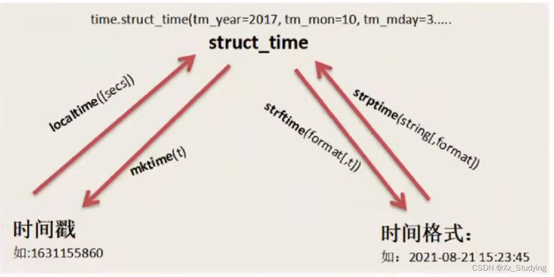
• timestamp 时间戳，时间戳表示的是从1970年1月1日 00：00：00开始按秒计算的偏移量
• struct_time 时间元组，共有九个元素组
• format time 格式化时间，已格式化的结构使时间更具有可读性。包括自定义格式和固定格式

时间格式转换图

# 导入 time 模块
import time
# 生成 timestamp
# print(int(time.time()))
# 程序开发时间
start_time = time.time()
 
# 程序
s =""
for i in range(10000):
    s += str(i)
    # sleep(睡眠多少秒)
    # time.sleep(1) # 程序暂停 1 秒
 
end_time = time.time()
print(f'程序消耗时间={end_time-start_time}')

运行结果:

程序消耗时间=0.002516508102416992

# 导入 time 模块
import time
# 生成struct_time
# timestamp to struct_time 本地时间
my_time = time.localtime()
print(f'my_time 为：{my_time}')
print(my_time.tm_year)
print(my_time.tm_mon)
print(my_time.tm_mday)
# 将timesstamp 转化为 struct_time
print(time.localtime(1650177058))
print(f'----------分割线-----------')
print(time.strftime('%Y-%m-%d'))    # 默认当前时间格式化
# 显示指定 struct_time 格式化后的时间
print(time.strftime('%Y-%m-%d', time.localtime(1650177058)))
print(time.strftime('%Y-%m-%d %X', time.localtime(1650177058)))
# 将格式化字符串到 struct_time,再转为时间戳
st = time.strptime('2011-05-05 16:37:06', '%Y-%m-%d %X')
print(time.mktime(st))
# 时间戳加 10 天
print(time.mktime(st) + 24*60*60*10)

运行结果：

my_time 为：time.struct_time(tm_year=2022, tm_mon=11, tm_mday=11, tm_hour=22, tm_min=6, tm_sec=2, tm_wday=4, tm_yday=315, tm_isdst=0)
2022
11
11
time.struct_time(tm_year=2022, tm_mon=4, tm_mday=17, tm_hour=14, tm_min=30, tm_sec=58, tm_wday=6, tm_yday=107, tm_isdst=0)
----------分割线-----------
2022-11-11
2022-04-17
2022-04-17 14:30:58
1304584626.0
1305448626.0

3.1.2 datetime 模块

        datetime 模块重新封装了 time 模块，提供更多接口，提供的类有：date, time, datetime, timedelta, tzinfo

1. date 类

datetime.date(year, month, day)

静态方法和字段

• date.today(): 返回一个表示当前本地日期的 date 对象
• date.fromtimestamp:  根据给定的时间戳，返回一个date 对象

from datetime import date
# 导入 time 模块
import time
print(f'date.today():{date.today()}')
print(f'date.fromtimestamp():{date.fromtimestamp(time.time())}')

运行结果：

date.today():2022-11-12
date.fromtimestamp():2022-11-12

from datetime import date
# 导入 time 模块
import time
now = date(2021, 10, 26)
print(now.year, now.month, now.day)
tomorrow = now.replace(day=1)
print(f'now:{now},当月第一天：{tomorrow}')
print(f'timetuple(): {now.timetuple()}')
print(f'weekday(): {now.weekday()}')
print(f'isoweekday(): {now.isoweekday()}')
print(f'isoformat(): {now.isoformat()}')
print(f'strftime(): {now.strftime("%Y.%m.%d")}')

 运行结果：

2021 10 26
now:2021-10-26,当月第一天：2021-10-01
timetuple(): time.struct_time(tm_year=2021, tm_mon=10, tm_mday=26, tm_hour=0, tm_min=0, tm_sec=0, tm_wday=1, tm_yday=299, tm_isdst=-1)
weekday(): 1
isoweekday(): 2
isoformat(): 2021-10-26
strftime(): 2021.10.26

2. datetime 类

datetime 相当于 date 和 time 结合起来

部分常用属性和方法：

// 通过datetime对象才能调用
dt.year、dt.month、dt.day：获取年、月、日；
dt.hour、dt.minute、dt.second、dt.microsecond：获取时、分、秒、微秒；
 
 
datetime.fromtimestamp():将时间戳转为一个datetime对象
dt.date()：获取date对象；
dt.time()：获取time对象；
dt.replace()：传入指定的year或month或day或hour或minute或second或microsecond，生成一个新日期datetime对象，但不改变原有的datetime对象；
dt.timetuple()：返回时间元组struct_time格式的日期； 
dt.weekday()：返回weekday，如果是星期一，返回0；如果是星期2，返回1，以此类推；
dt.isoweekday()：返回weekday，如果是星期一，返回1；如果是星期2，返回2，以此类推；
dt.isocalendar()：返回(year,week,weekday)格式的元组；
dt.isoformat()：返回固定格式如'YYYY-MM-DD HH:MM:SS’的字符串
dt.strftime(format)：传入任意格式符，可以输出任意格式的日期表示形式。

from datetime import datetime
# 导入 time 模块
import time
now = datetime.now()
print(type(now))
# 将datetime 转化为指定格式的字符串
print(now.strftime('%Y-%m-%d %X'))
print(now.strftime('%Y-%m-%d %H:%M'))
# '2021-11-10 10:23'，使用strptime 将字符串转 datetime(格式要统一)
my_str = '2021-11-10 10:23'
print(datetime.strptime(my_str, '%Y-%m-%d %H:%M'))
print(f'获取date对象:{now.date()}')
print(f'获取time对象:{now.time()}')
print(f'返回时间元组struct_time格式的日期:{now.timetuple()}')

运行结果：

<class 'datetime.datetime'>
2022-11-12 16:43:13
2022-11-12 16:43
2021-11-10 10:23:00
获取date对象:2022-11-12
获取time对象:16:43:13.423626
返回时间元组struct_time格式的日期:time.struct_time(tm_year=2022, tm_mon=11, tm_mday=12, tm_hour=16, tm_min=43, tm_sec=13, tm_wday=5, tm_yday=316, tm_isdst=-1)

3.1.3 timedelta 类，时间加减

        使用 timedelta 可以很方便的在日期上做天 days，小时 hour，分钟，秒，毫秒，微妙的时间计算，如果要计算月份则需要另外的办法

from datetime import datetime
from datetime import timedelta
dt = datetime.now()
# 日期减一天
dt_1 = dt + timedelta(days=-1)  # 昨天
dt_2 = dt - timedelta(days=1)  # 昨天
dt_3 = dt + timedelta(days=1)  # 明天
print(f'今天：{dt}')
print(f'昨天：{dt_1}')
print(f'昨天：{dt_2}')
print(f'明天：{dt_3}')
# 明天的 datetime- 昨天的datetime
s =dt_3 - dt_1
print(f'相差的天数：{s.days}')
print(f'相差的秒数：{s.total_seconds()}')

运行结果：

今天：2022-11-12 17:05:10.986492
昨天：2022-11-11 17:05:10.986492
昨天：2022-11-11 17:05:10.986492
明天：2022-11-13 17:05:10.986492
相差的天数：2
相差的秒数：172800.0

3.2 Pandas 时间 Timedelta

        表示持续时间，即两个日期或时间之间的差异。

        相当于 python 的datetime.timedelta ,在大多数情况下可以与之互换

import time
 
import pandas as pd
from datetime import datetime
from datetime import timedelta
ts = pd.Timestamp('2022-11-12 12')
print(ts)
# 减一天
print(f'减去一天后：{ts + pd.Timedelta(-1, "D")}')
# 时间间隔
td = pd.Timedelta(days=5, minutes=50, seconds=20)   # 关键字赋值
print(f'ts + td ={ts + td}')
print(f'总秒数：{td.total_seconds()}')
 

运行结果：

2022-11-12 12:00:00
减去一天后：2022-11-11 12:00:00
ts + td =2022-11-17 12:50:20
总秒数：435020.0

3.3 Pandas 时间转化 to_datetime

        to_datetime 转换时间戳，可以通过 to_datetime 能快速将字符串转换为时间戳。当传递一个 Series 时，它会返回一个 Series（具有相同的索引），而类似列表的则转换为 DatetimeIndex

 

import pandas as pd
df = pd.DataFrame({'year': [2015, 2016], 'month': [2, 3], 'day': [4, 5]})
print(df)
print(f'pd.Datetime(df):\n{pd.to_datetime(df)}')
# 将字符串转为 datetime
print(pd.to_datetime(['11-12-2021']))
print(pd.to_datetime(['2005/11/13', "2010.12.31"]))
# 除了可以将文本数据转换为时间戳外，还可以将 unix 时间转换为时间戳
print(pd.to_datetime([1349720105, 1349806505, 1349892905], unit="s"))
# 自动识别异常
print(pd.to_datetime('210605'))
print(pd.to_datetime('210605', yearfirst=True))
# 配合 uint 参数，使用非unix 时间
print(pd.to_datetime([1, 2, 3], unit='D', origin=pd.Timestamp('2020-01-11')))
print(pd.to_datetime([1, 2, 3], unit='d'))
print(pd.to_datetime([1, 2, 3], unit='h', origin=pd.Timestamp('2020-01')))
print(pd.to_datetime([1, 2, 3], unit='m', origin=pd.Timestamp('2020-01')))
print(pd.to_datetime([1, 2, 3], unit='s', origin=pd.Timestamp('2020-01')))

 运行结果：

   year  month  day
0  2015      2    4
1  2016      3    5
pd.Datetime(df):
0   2015-02-04
1   2016-03-05
dtype: datetime64[ns]
DatetimeIndex(['2021-11-12'], dtype='datetime64[ns]', freq=None)
DatetimeIndex(['2005-11-13', '2010-12-31'], dtype='datetime64[ns]', freq=None)
DatetimeIndex(['2012-10-08 18:15:05', '2012-10-09 18:15:05',
               '2012-10-10 18:15:05'],
              dtype='datetime64[ns]', freq=None)
2005-06-21 00:00:00
2021-06-05 00:00:00
DatetimeIndex(['2020-01-12', '2020-01-13', '2020-01-14'], dtype='datetime64[ns]', freq=None)
DatetimeIndex(['1970-01-02', '1970-01-03', '1970-01-04'], dtype='datetime64[ns]', freq=None)
DatetimeIndex(['2020-01-01 01:00:00', '2020-01-01 02:00:00',
               '2020-01-01 03:00:00'],
              dtype='datetime64[ns]', freq=None)
DatetimeIndex(['2020-01-01 00:01:00', '2020-01-01 00:02:00',
               '2020-01-01 00:03:00'],
              dtype='datetime64[ns]', freq=None)
DatetimeIndex(['2020-01-01 00:00:01', '2020-01-01 00:00:02',
               '2020-01-01 00:00:03'],
              dtype='datetime64[ns]', freq=None)

3.4  Pandas 时间序列 date_range        

        有时候，我们可能想要生成某个范围内的时间戳。例如，我想要生成“2018-6-26” 这一天之后的 8 天时间戳，我们可以使用 date_range 和 bdate_range 来完成时间戳范围的生成。

import pandas as pd
# 指定默认值，默认时包含开始和结束时间，默认频率使用的D（天）
print(pd.date_range(start='1/1/2021', end='1/08/2021'))
print(pd.date_range(start='2010', end='2011'))
# 指定开始日期，设置期间数
print(pd.date_range(start='1/1/2018', periods=8))
# 指定开始、结束和期间；频率自动生成（线性间隔）
print(pd.date_range(start='2018-04-24', end='2018-04-27', periods=3))
print(pd.date_range(start='2018-04-24', end='2018-04-27', periods=4))
print(pd.date_range(start='2018-04-24', periods=4))
print(pd.date_range(start='2018-04-24 15:30', periods=4, name='mypd'))
print(pd.date_range(start='2018-04-24 15:30', periods=4, name='mypd', normalize=True))

 运行结果：

DatetimeIndex(['2021-01-01', '2021-01-02', '2021-01-03', '2021-01-04',
               '2021-01-05', '2021-01-06', '2021-01-07', '2021-01-08'],
              dtype='datetime64[ns]', freq='D')
DatetimeIndex(['2010-01-01', '2010-01-02', '2010-01-03', '2010-01-04',
               '2010-01-05', '2010-01-06', '2010-01-07', '2010-01-08',
               '2010-01-09', '2010-01-10',
               ...
               '2010-12-23', '2010-12-24', '2010-12-25', '2010-12-26',
               '2010-12-27', '2010-12-28', '2010-12-29', '2010-12-30',
               '2010-12-31', '2011-01-01'],
              dtype='datetime64[ns]', length=366, freq='D')
DatetimeIndex(['2018-01-01', '2018-01-02', '2018-01-03', '2018-01-04',
               '2018-01-05', '2018-01-06', '2018-01-07', '2018-01-08'],
              dtype='datetime64[ns]', freq='D')
DatetimeIndex(['2018-04-24 00:00:00', '2018-04-25 12:00:00',
               '2018-04-27 00:00:00'],
              dtype='datetime64[ns]', freq=None)
DatetimeIndex(['2018-04-24', '2018-04-25', '2018-04-26', '2018-04-27'], dtype='datetime64[ns]', freq=None)
DatetimeIndex(['2018-04-24', '2018-04-25', '2018-04-26', '2018-04-27'], dtype='datetime64[ns]', freq='D')
DatetimeIndex(['2018-04-24 15:30:00', '2018-04-25 15:30:00',
               '2018-04-26 15:30:00', '2018-04-27 15:30:00'],
              dtype='datetime64[ns]', name='mypd', freq='D')
DatetimeIndex(['2018-04-24', '2018-04-25', '2018-04-26', '2018-04-27'], dtype='datetime64[ns]', name='mypd', freq='D')