2.5 Regression

2.5 Regression

Question 1

Which of the following items does not apply to the sum of squared residuals (SSR) from an ordinary least square (OLS) regression?

A. SSR is equal to $\sum e_i^2$
B. SSR is equal to $\sum [Y_i-(b_0+b_1{X}_i)]$
C. When using OLS, SSR is minimized
D. SSR can indicate how well the regression model explains the dependent variable

Answer: B
Total sum of squares(TSS): sum of squared deviations of $Y_i$ from its average.
$TSS={\sum }_{i=1}^n(Y_i-\overline{Y}{)}^2$
Explained sum of squares(ESS): sum of squared deviations of the predicted values $\widehat{Y_i}$.
$ESS={\sum }_{i=1}^n(\widehat{Y_i}-\overline{Y}{)}^2$
Residual Sum of squares(RSS): sum of squared residuals or the residual of squares.
$RSS={\sum }_{i=1}^n(Y_i-\widehat{Y_i}{)}^2={\sum }_{i=1}^n{e}_i^2={\sum }_{i=1}^n[Y_i-(b_0+b_1{X}_i){]}^2$

Ordinary least squares(OLS) estimation is a process that minimize the square deviations between the realizations of the dependent variable $Y$ and their expected values given the respective realization of $X$. In turn, these estimators minimize the residual sum of squares.

---

Question 2

An analyst is using a statistical package to perform a linear regression between the risk and return from securities in an emerging market country. The original data and intermediate statistics are shown on the right. The value of coefficient of determination for this regression is closest to:

A. $0.043$
B. $0.084$
C. $0.916$
D. $0.957$

Answer: C: Coefficient determination

${\mu }_x=3.5$, ${\mu }_y=4.3$

${\sum }_{i=1}^7(x_i-{\mu }_x{)}^2=24.9$, ${\sum }_{j=1}^7(y_j-{\mu }_y{)}^2=3.63$, ${\sum }_{i=j1}^7(x_i-{\mu }_x)(y_j-{\mu }_y)=9.1$

$R^2={\rho }^2=\frac{Cov(X,Y{)}^2}{{\sigma }_x^2{\sigma }_y^2}=0.916$

• For simple linear regression, $R^2$ is equal to the correlation coefficient.
• $R^2$ measures the percentage of the variation in the data that can be explained by the model.
• Because OLS estimates parameters by finding the values that minimize the RSS, the OLS estimator also maximizes $R^2$.

---

Question 3

PE2018Q17 / PE2019Q17 / PE2020Q17 / PE2021Q17 / PE2022PSQ16 / PE2022Q17
The proper selection of factors to include in an ordinary least squares estimation is critical to the accuracy of the result. When does omitted variable bias occur?

A. Omitted variable bias occurs when the omitted variable is correlated with the included regressor and is a determinant of the dependent variable.
B. Omitted variable bias occurs when the omitted variable is correlated with the included regressor but is not a determinant of the dependent variable.
C. Omitted variable bias occurs when the omitted variable is independent of the included regressor and is a determinant of the dependent variable,
D. Omitted variable bias occurs when the omitted variable is independent of the included regressor but is not a determinant of the dependent variable.

Answer: A
Learning Objective: Describe the consequences of excluding a relevant explanatory variable from a model and contrast those with the consequences of including an irrelevant regressor.

Omitted variable bias occurs when a model improperly omits one or more variables that are critical determinants of the dependent variable and are correlated with one or more of the other included independent variables. Omitted variable bias results in an over- or under-estimation of the regression parameters.

---

Question 4

Using standard Monte Carlo methods, an analyst prices a European call options using $1,000$ simulations of underlying stock price. The option price is estimated at USD $1.00$ with a standard error USD $0.40$. All other things kept constant. If the analyst increases the number of simulations to $3,000$, the resulting standard error is likely to be:

A. $0.13$
B. $0.21$
C. $0.23$
D. $0.69$

Answer: C
$SE=\mu /\sqrt{n}$

• The standard deviation of the mean estimator (or any other estimator) is known as a standard error.
• Standard errors are important in hypothesis testing and when performing Monte Carlo simulations. In both of these applications, the standard error provides an indication of the accuracy of the estimate.

---

Question 5

Which of the following is most likely in the case of high multicollinearity?

A. Low F ratio and insignificant partial slope coefficients
B. High F ratio and insignificant partial slope coefficients
C. Low F ratio and significant partial slope coefficients
D. High F ratio and significant partial slope coefficients

Answer: B
Classic symptom of high multicollinearity is high R2 (corresponds to high F ratio) but insignificant partial slope coefficients.

---

Question 6

Which of the following statements is correct regarding the use of the F-test and the F-statistic?

I. For simple linear regression, the F-test tests the same hypothesis as the t-test.
II. The F-statistic is used to find which items in a set of independent variables explain a significant portion of the variation of the dependent variable.

A. I only
B. II only
C. Both I and II
D. Neither I nor II

Answer: A
The simple linear regression F-test tests the same hypothesis as the t-test because there is only one independent variable.

An F-test is used to test whether at least one slope coefficient
is significantly different from zero.

The F-statistic is used to tell you if at least one independent variable in a set of independent variables explains a significant portion of the variation of the dependent variable. It tests the independent variables as a group, and thus won’t tell you which variable has significant explanatory power.

---

Question 7

Greg Barns, FRM, and Jill Tillman, FRM, are discussing the hypothesis they wish to test with respect to the model represented by $Y_i=B_0+B_1{X}_i+{\epsilon }_i$. They wish to use the standard statistical methodology in their test. Barns thinks an appropriate hypothesis would be that $B_1=0$ with the goal of proving it to be true. Tillman thinks an appropriate hypothesis to test is $B_1=1$ with the goal of rejecting it. With respect to these hypotheses:

A. The hypothesis of neither researcher is appropriate.
B. The hypothesis of Barns is appropriate but not that of Tillman.
C. The hypothesis of Tillman is appropriate but not that of Barns.
D. More information is required before a hypothesis can be set up.

Answer: C
The usual approach is to specify a hypothesis that the researcher wishes to disprove.

---

Question 8

Which one of the following statements about the correlation coefficient is false?

A. It always ranges from $-1$ to $+1$.
B. A correlation coefficient of zero means that two random variables are independent.
C. It is a measure of linear relationship between two random variables.
D. It can be calculated by scaling the covariance between two random variables.

Answer: B
Correlation describes the linear relationship between two variables. While we would expect to find a correlation of zero for independent variables, finding a correlation of zero does not mean that two variables are independent.

---

Question 9

The correlation coefficient for two dependent random variables is equal to:

A. the product of the standard deviations for the two random variables divided by the covariance.
B. the covariance between the random variables divided by the product of the variances.
C. the absolute value of the difference between the means of the two variables divided by the product of the variances.
D. the covariance between the random variables divided by the product of the standard deviations

Answer: D
$\rho =\frac{Cov(x,y)}{{\sigma }_x{\sigma }_y}$

---

Question 10

Consider two shock, A and B. Assume their annual returns are jointly normally distributed, the marginal distribution of each stock has mean $2\%$ and standard deviation $20\%$, and the correlation is $0.9$. What is the expected annual return of stock A if the annual return of stock B is $3\%$.

A. $2\%$
B. $2.9\%$
C. $4.7\%$
D. $1.1\%$

Answer: B
The information in this question can be used to construct a regression model of A on B.

We have $R_A=b_0+b_1{R}_B+ϵ$

$b_1=\frac{Cov(A,B)}{{\sigma }_A^2}=\frac{\rho {\sigma }_A{\sigma }_B}{{\sigma }_A^2}=0.9$, $b_0=\overline{R_A}-b_1\overline{R_B}=0.002$

---

Question 11

PE2018Q8 / PE2019Q8
An analyst is trying to get some insight into the relationship between the return on stock LMD and the return on the S&P 500 index. Using historical data she estimates the following:

Annual mean return for LMD is $11\%$
Annual mean return for S&P 500 index is $7\%$
Annual volatility for S&P 500 index is $18\%$
Covariance between the returns of LMD and S&P 500 index is $6\%$

Assuming she uses the same data to estimate the regression model given by:

$$R_{\text{LMD,t}}=\alpha +\beta \times R_{\text{SP500,t}}+{ϵ}_t$$

Using the ordinary least squares technique, which of the following models will the analyst obtain?

A. $R_{\text{LMD,t}}=-0.02+0.54\times R_{\text{SP500,t}}+ϵ$
B. $R_{\text{LMD,t}}=-0.02+1.85\times R_{\text{SP500,t}}+ϵ$
C. $R_{\text{LMD,t}}=0.04+0.54\times R_{\text{SP500,t}}+ϵ$
D. $R_{\text{LMD,t}}=0.04+1.85\times R_{\text{SP500,t}}+ϵ$

Answer: B
Learning Objective: Explain how regression analysis in econometrics measures the relationship between dependent and independent variables.

The regression coefficients for a model specified by $Y=bX+a+ϵ$ are obtained using the formulas:

$b=Cov(X,Y)/{\sigma }_X^2$, $a=E(Y)-b\times E(X)$

Then: $b=0.06/(0.18{)}^2=1.85$, $a=0.11-(1.85\times 0.07)=-0.02$

---

Question 12

Which of the following is assumed in the multiple least squares regression model?

A. The dependent variable is stationary.
B. The independent variables are not perfectly multicollinear.
C. The error terms are heteroskedastic.
D. The independent variables are homoskedastic.

Answer:B
Extending the model to multiple regressors requires one additional assumption, along with some modifications, to the five assumptions in simple linear regression.

• The explanatory variables are not perfectly linearly dependent.
• All variables must have positive variances so that ${\sigma }_{X_j}^2>0$ for $j=1,2,\cdots ,k$.
• The random variables ($Y_i,X_{1i},X_{2i},\cdots ,X_{Ki}$) are assumed to be iid.
• The error is assumed to have mean zero conditional on the explanatory variables (i.e. $E[{ϵ}_i|X_{1i},X_{2i},\cdots ,X_{Ki}=0$).
• The constant variance assumption is similarly extended to hold for all explanatory variables (i.e. $E[{ϵ}_i^2|X_{1i},X_{2i},\cdots ,X_{Ki}={\sigma }^2$).
• No outliers.

---

Question 13

Which of the following statements about the ordinary least squares regression model (or simple regression model) with one independent variable are correct?

I. In the ordinary least squares (OLS) model, the random error term is assumed to have zero mean and constant variance.
II. In the OLS model, the variance of the independent variable is assumed to be positively correlated with the variance of the error term.
III. In the OLS model, it is assumed that the correlation between the dependent variable and the random error term is zero.
IV. In the OLS model, the variance of the dependent variable is assumed to be constant.

A. I, II, III and IV
B. Il and IV only
C. I and IV only
D. I, II, and Ill only

---

Question 14

PE2018Q42 / PE2019Q42 / PE2020Q42 / PE2021Q42 / P2022Q42
A risk manager performs an ordinary least squares (OLS) regression to estimate the sensitivity of a stock’s return to the return on the S&P 500. This OLS procedure is designed to:

A. Minimize the square of the sum of differences between the actual and estimated S&P 500 returns.
B. Minimize the square of the sum of differences between the actual and estimated stock returns.
C. Minimize the sum of differences between the actual and estimated squared S&P 500 returns.
D. Minimize the sum of squared differences between the actual and estimated stock returns.

Answer: D
Learning Objective: Define an ordinary least squares (OLS) regression and calculate the intercept and slope of the regression.

The OLS procedure is a method for estimating the unknown parameters in a linear regression model.

The method minimizes the sum of squared differences between the actual, observed, returns and the returns estimated by the linear approximation. The smaller the sum of the squared differences between observed and estimated values, the better the estimated regression line fits the observed data points.

---

Question 15

PE2018Q44 / PE2019Q44
Using data from a pool of mortgage borrowers, a credit risk analyst performed an ordinary least squares regression of annual savings (in GBP) against annual household income (in GBP) and obtained the following relationship:

$\text{Annual Savings}=0.24\times \text{Household Income}-25.66,R^2=0.50$

Assuming that all coefficients are statistically significant, which interpretation of this result is correct?

A. For this sample data, the average error term is GBP $-25.66$.
B. For a household with no income, annual savings is GBP $0$.
C. For an increase of GBP 1,000 in income, expected annual savings will increase by GBP $240$.
D. For a decrease of GBP 2,000 in income, expected annual savings will increase by GBP $480$.

Answer: C
Learning Objective: Interpret a population regression function, regression coefficients, parameters, slope, intercept, and the error term.

An estimated coefficient of $0.24$ from a linear regression indicates a positive relationship between income and savings, and more specifically means that a one unit increase in the independent variable (household income) implies a $0.24$ unit increase in the dependent variable (annual savings). Given the equation provided, a household with no income would be expected to have negative annual savings of GBP $25.66$. The error term mean is assumed to be equal to $0$.

---

Question 16

You are conducting an ordinary least squares regression of the returns on stocks $Y$ and $X$ as $Y=a+bxX+ϵ$ based on the past three year’s daily adjusted closing price data. Prior to conducting the regression, you calculated the following information from the data:

Sample covariance is $0.000181$
Sample Variance of Stock $X$ is $0.000308$
Sample Variance of Stock $Y$ is $0.000525$
Sample mean return of stock $X$ is $-0.03\%$
Sample mean return of stock $Y$ is $0.03\%$

What is the slope of the resulting regression line?

A. $0.35$
B. $0.45$
C. $0.59$
D. $0.77$

---

Question 17

Paul Graham, FRM is analyzing the sales growth of a baby product launched three years ago by a regional company. He assesses that three factors contribute heavily towards the growth and comes up with the following results:

$Y=b+1.5\times X_1+1.2\times X_2+3\times X_3$
Sum of Squared Regression, $SSR=869.76$
Sum of Squared Errors, $SEE=22.12$

Determine what proportion of sales growth is explained by the regression results.

A. $0.36$
B. $0.98$
C. $0.64$
D. $0.55$

Answer: B
Sum of squared regression also means explained sum of squares.

$R^2=ESS/TSS=1-SSR/TSS$

---

Question 18

A regression of a stock’s return (in percent) on an industry index’s return (in percent) provides the following results:

Which of the following statements regarding the regression is correct?

I. The correlation coefficient between the X and Y variables is $0.889$.
II. The industry index coefficient is significant at the $99\%$ confidence interval.
III. If the return on the industry index is $4\%$, the stock’s expected return is $10.3\%$.
IV. The variability of industry returns explains $21\%$ of the variation of company returns.

A. IIl only
B. I and II only
C. Il and IV only
D. I, II, and IV

Answer: B
The $R^2$ of the regression is calculated as $ESS/TSS=(92.648/117.160)=0.79$, which means that the variation in industry returns explains $79\%$ of the variation in the stock return. By taking the square root of $R^2$, we can calculate that the correlation coefficient $\rho =0.889$.

The t-statistic for the industry return coefficient is $1.91/0.31=6.13$, which is sufficiently large enough for the coefficient to be significant at the $99\%$ confidence interval.

Since we have the regression coefficient and intercept, we know that the regression equation is $R_{stock}=1.9\times X+2.1$. Plugging in a value of 4% for the industry return, we get a stock return of $1.9\times 4\%+2.1=9.7\%$.

---

Question 19

An analyst is given the data in the following table for a regression of the annual sales for Company XYZ, a maker of paper products, on paper product industry sales.

The correlation between company and industry sales is 0.9757. Which of the following is closest to the value and reports the most likely interpretation of the $R^2$?

A. $0.048$, indicating that the variability of industry sales explains about $4.8\%$ of the variability of company sales.
B. $0.048$, indicating that the variability of company sales explains about $4.8\%$ of the variability of industry sales.
C. $0.952$, indicating that the variability of industry sales explains about $95.2\%$ of the variability of company sales.
D. $0.952$, indicating that the variability of company sales explains about $95.2\%$ of the variability of industry sales.

---

Question 20

PE2018Q9 / PE2019Q9 / PE2020Q9 / PE2021Q9 / PE2022Q9
For a sample of $400$ firms, the relationship between corporate revenue ($Y_i$) and the average years of experience per employee ($X_i$) is modeled as follows:

$Y_i={\beta }_1+{\beta }_2{X}_i+{ϵ}_i,i=1,2,\cdots ,400$

An analyst wish to test the joint null hypothesis that at the $95\%$ confidence level. The p-value for the t-statistic for ${\beta }_1$ is $0.07$, and the p-value for the t-statistic for ${\beta }_2$ is $0.06$. The p-value for the F-statistic for the regression is $0.045$. Which of the following statements is correct?

A. The analyst can reject the null hypothesis because each $\beta$ is different from $0$ at the $95\%$ confidence level.
B. The analyst cannot reject the null hypothesis because neither $\beta$ is different from $0$ at the $95\%$ confidence level.
C. The analyst can reject the null hypothesis because the F-statistic is significant at the $95\%$ confidence level.
D. The analyst cannot reject the null hypothesis because the F-statistic is not significant at the $95\%$ confidence level.

Answer: C
Learning Objective: Construct, apply and interpret joint hypothesis tests and confidence intervals for multiple coefficients in a regression.

The T-test would not be sufficient to test the joint hypothesis. In order to test the joint null hypothesis, examine the F-statistic, which in this case is statistically significant at the $95\%$ confidence level. Thus the null can be rejected.

---

Question 21

Use the following information to answer the following question.

Based on the results and a $5\%$ level of significance, which of the following hypotheses can be
rejected?
I. $H_0:B_0=0$
II. $H_0:B_1=0$
III. $H_0:B_2=0$
IV. $H_0:B_1=B_2=0$

A. I, II, and III
B. I and IV
C. Ill and IV
D. I, IIl, and IV

Answer: D
The t-statistics for the intercept and coefficient on are significant as indicated by the associated p-values being less than $0.05$: $0.0007$ and $0.0004$ respectively. Therefore, $H_0:B_0=0$ and $H_0:B_2=0$ can be rejected.

The F-statistic on the ANOVA table has a p-value equal to $0.0012$; therefore, $H_0:B_1=B_2=0$ can be rejected.

---

Question 22

PE2018Q26 / PE2019Q26 / PE2020Q26 / PE2021Q26 / PE2022Q26
A risk manager has estimated a regression of a firm’s monthly portfolio returns against the returns of three U.S. domestic equity indexes: the Russell 1000 index, the Russell 2000 index, and the Russell 3000 index. The results are shown below.

Based on the regression results, which statement is correct?

A. The estimated coefficient of $0.3533$ indicates that the returns of the Russell 3000 index are more statistically significant in determining the portfolio returns than the other two indexes.
B. The high adjusted $R^2$ indicates that the estimated coefficients on the Russell 1000, Russell 2000, and Russell 3000 indexes are statistically significant.
C. The high p-value of $0.9452$ indicates that the regression coefficient of the returns of Russell 1000 is more statistically significant than the other two indexes.
D. The high correlations between each pair of index returns indicate that multicollinearity exists between the variables in this regression.

Answer: D
Learning Objective:

• Interpret regression coefficients in a multiple regression,
• Interpret goodness of fit measures for single and multiple regressions, including $R^2$ and adjusted $R^2$.
• Characterize multicollinearity and its consequences; distinguish between multicollinearity and perfect collinearity.

This is an example of multicollinearity, which arises when one of the regressors is very highly correlated with the other regressors. In this case, all three regressors are highly correlated with each other, so multicollinearity exists between all three. Since the variables are not perfectly correlated with each other this is a case of imperfect, rather than perfect, multicollinearity.

---

Question 23

PE2018Q28 / PE2019Q28 / PE2020Q28 / PE2021Q28 / PE2022Q28
An analyst is testing a hypothesis that the beta, $\beta$, of stock CDM is $1$. The analyst runs an ordinary least squares regression of the monthly returns of CDM, $R_{CDM}$, on the monthly returns of the S&P 500 index, $R_m$, and obtains the following relation:
$$R_{CDM}=0.86\times R_m-0.32$$

The analyst also observes that the standard error of the coefficient of $R_m$ is $0.80$. In order to test the hypothesis $H_0:\beta =1$ against $H_1:\beta \ne 1$, what is the correct statistic to calculate?

A. t-statistic
B. Chi-square test statistic
C. Jarque-bera test statistic
D. Sum of squared residuals

Answer: A
Learning Objective:

• Construct, apply and interpret hypothesis tests and confidence intervals for a single regression coefficient in a regression.
• Explain the steps needed to perform a hypothesis test in a linear regression.

The t-statistic is defined by:
$$t=\frac{{\beta }^{\text{estimated}}-\beta }{S{E}_{\text{estimated }\beta }}=\frac{0.86-1}{0.8}=-0.175$$

In the case $t=-0.175$. Since $|t|<1.96$, we cannot reject the null hypothesis.

---

Question 24

A bank analyst run an ordinary least squares regression of the daily returns of the stock on the daily returns on the S&P 500 index using the last $750$ trading days of data. The regression results are summarized in the following tables:

The bank analyst wants to test the null hypothesis that the beta of the portfolio is $1.3$ at a $5\%$ significance level. According to the regression results, the analyst would:

A. Reject the null hypothesis because the t-statistic is greater than $1.96$.
B. Fail to reject the null hypothesis because the t-statistic is greater than $1.96$.
C. Reject the null hypothesis because the p-value is greater than $5\%$.
D. Fail to reject the null hypothesis because the p-value is greater than $5\%$.

---

Question 25

Many statistical problems arise when estimating relationships using regression analysis. Some of these problems are due to the assumptions behind the regression model. Which one of the following is NOT one of these problems?

A. Stratification
B. Multicollinearity
C. Heteroscedasticity
D. Autocorrelation

Answer: A
Stratification is not related to regression analysis. Choices B, C, and D describe situations that can produce inaccurate descriptions of the relationship between the independent and dependent variables.

Multicollinearity occurs when the independent variables are themselves correlated.
Heteroscedasticity occurs when the variances are different across observations.
Autocorrelation occurs when successive observations are influenced by the proceeding observations.

---

Question 26

An analyst is performing a regression. The dependent variable is portfolio return while the independent variable is the years of experience of the portfolio manager. In his analysis, the resulting scatter plot is as follow; The analyst can conclude that the portfolio returns exhibit:

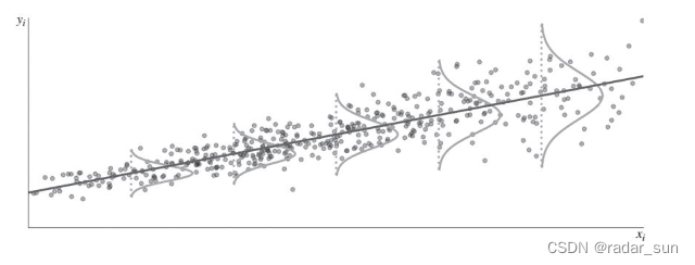
A. Heteroskedasticity
B. Homoskedasticity
C. Perfect multicollinearity
D. Non-perfect multicollinearity

---

Question 27

A risk manager is examining the relationship between portfolio manager’s years of working experience and the returns of their portfolios. He performs an ordinary least squares(OLS) regression of last year’s portfolio returns ($Y$) on the portfolio managers’ years of working experience($X$) and provides the following scatter plot to his supervisor:

Which of the following assumptions of the OLS regression has most likely been violated?

A. Perfect multicollonearity
B. Expectation of zero for the error terms
C. Normally distributed error terms
D. Homoskedasticity

---

Question 28

PE2022PSQ12
A risk manager at Firm SPC is testing a portfolio for heteroskedasticity using the White test. The portfolio is modeled as follows:

$$Y=\alpha +\beta \times X+ϵ$$

The residuals are computed as follows:

$$\widehat{ϵ}=Y_i-\hat{a}-b\times X_{1i}$$

Which of the following correctly depicts the second step in the White test for the portfolio?

A. ${\widehat{ϵ}}^2={\gamma }_0+{\gamma }_1{X}_{1i}+{\gamma }_2{X}_{1i}^2+\eta$
B. ${\widehat{ϵ}}^2={\gamma }_1{X}_{1i}+{\gamma }_2{X}_{1i}^2+\eta$
C. ${\widehat{ϵ}}^2={\gamma }_0+{\gamma }_1{X}_{1i}+\eta$
D. ${\widehat{ϵ}}^2={\gamma }_0+{\gamma }_1{X}_{1i}^2+\eta$

Answer: A
Learning Objective: Explain how to test whether a regression is affected by heteroskedasticity.

A is correct. The second step in the White test is to regress the squared residuals on a constant, on all explanatory variables, and on the cross product of all explanatory variables.

B is incorrect. It is missing the constant.

C is incorrect. It is missing the cross-product.

D is incorrect. It is missing the explanatory variable.

---

Question 29

The portfolio manager is interested in the systematic risk of a stock portfolio, so he estimates the linear regression: $R_p-R_f=\alpha +\beta (R_m-R_f)+ϵ$, where $R_p$ is the return of the portfolio at time $t$, $R_m$ is the return of the market portfolio at time $t$, and $R_f$ is the risk-free rate, which is constant over time. Suppose that $\alpha =0.0008$, $\beta =0.977$, $\sigma (R_p)=0.167$ and $\sigma (R_m)=0.156$, What is the approximate coefficient of determination in this regression?

A. $0.913$
B. $0.834$
C. $0.977$
D. $0.955$

Answer: B
$R^2={\rho }^2={\left[\frac{\text{Cov}(R_p,R_m)}{{\sigma }_{R_p}{\sigma }_{R_m}}\right]}^2$, and $\text{Cov}(R_p,R_m)=\beta \times {\sigma }_{R_m}^2$

Thus, $R^2={\left[\frac{\beta \times {\sigma }_{R_m}}{{\sigma }_{R_p}}\right]}^2={\left[\frac{0.977\times 0.156}{0.167}\right]}^2=0.83$

---

Question 30

Consider the following linear regression model: $Y=a+bX+ϵ$. Suppose $a=0.05$, $b=1.2$, $SD(Y)=0.26$, $SD(e)=0.1$. What is the correlation between $X$ and $Y$?

A. $0.923$
B. $0.852$
C. $0.701$
D. $0.462$

Answer: A
$V(Y)=b^{2}V(X)+V(ϵ)\to V(X)=0.04\to SE(X)=0/2$

$\rho =\frac{\text{Cov}(X,Y)}{{\sigma }_x{\sigma }_y}=\frac{b\times SE(X)}{SE(Y)}=0.923$

---

Question 31

Our linear regression produces a high coefficient of determination ($R^2$ ) but few significant t ratios. Which assumption is most likely violated?

A. Homoscedasticity
B. Multicollinearity
C. Error term is normal with mean = 0 and constant variance = sigma2
D. No autocorrelation between error terms

Answer: B
High $R^2$ (implies F test will probably reject null) but low significance of partial slope coefficients is the classic symptom of multicollinearity.