R语言---PCA/tSNE/UMAP降维计算

目前，需要将不同材料的基因型数据降维，使用线性降维方法PCA，非线性降维方法tSNE和UMAP。
使用的输入输入数据是不同材料基因型的相似性矩阵，期望获得多个SNP，不同材料的降维情况。

1. PCA计算

PCA（principal component analysis）是一种线性降维方法，通常分为R-mode和Q-mode，数据列为variable，行为unit；在R语言中计算PCA，常用princomp和prcomp函数。

(1) princomp函数

princomp函数是基于协方差(covariance) 或者相关矩阵(correlation) 提取的特征(eigen)并进行特征值分解。
princomp函数适用行数大于列数的数据（即 units数目大于variables数目），否则报错：

> x=t(mtcars)
> dim(x)
[1] 11 32
> princomp(x)
Error in princomp.default(x) : 
  'princomp' can only be used with more units than variables
1
2
3
4
5
6

默认参数为：

## Default S3 method:
princomp(x, cor = FALSE, scores = TRUE, covmat = NULL,
         subset = rep_len(TRUE, nrow(as.matrix(x))), fix_sign = TRUE, ...)
1
2
3

在R中键入?princomp，会发现该函数推荐我们使用prcomp：

The calculation is done using eigen on the correlation or covariance matrix, 
as determined by cor. This is done for compatibility with the S-PLUS result. 
A preferred method of calculation is to use svd on x, as is done in prcomp.
1
2
3

princomp PCA结果：

pca_iris = princomp(iris[,1:4])$scores[,1:2]
plot(pca_iris, t='n')
text(pca_iris, labels=iris$Species,col=colors[iris$Species])
1
2
3

(2) prcomp函数

prcomp函数的计算是基于奇异值分解的（singular value decomposition，svd），对于R/Q-mode数据都可以，不会报错，因此比上面的函数更好用。
默认参数为：

## Default S3 method:
prcomp(x, retx = TRUE, center = TRUE, scale. = FALSE,
       tol = NULL, rank. = NULL, ...)
1
2
3

该函数有两个参数比较重要：

scale.  =  TRUE/FALSE (default FALSE)
center  = TRUE/FALSE (default TRUR)
1
2

scale. 这个参数通常设置为TRUE，因为这样可以对数据框进行scale（zscore标准化），防止因为数据的数量级不同对结果产生影响。当然了这个参数设置FALSE，但传入的是预先scale的数据是不影响结果的。
实际情况，还是要看啊，具体并不能确定哪个更好（scale. =T/F）。

使用自带的iris数据框计算举例：

## prcomp method：简单出图版本
pca.res <- prcomp(iris[,1:4])$x[,1:2]
plot(pca.res, t='n')
text(pca.res, labels=iris$Species,col=colors[iris$Species])
1
2
3
4

##  prcomp method：计算percentage
pca.res <- prcomp(iris[,1:4])
summary(pca.res)
pca.plot=as.data.frame(pca.res$x[,1:2])
colnames(pca.plot)=c("PC1","PC2")
## calculate percentage 
percent = round(pca.res$sdev^2/sum(pca.res$sdev^2), 4)
pc1r=percent[1]
pc2r=percent[2]

plot(pca.plot, t='n',xlab=paste("PC1","(",round(pc1r * 100, 2),"%)"),
     ylab=paste("PC2","(",round(pc2r * 100, 2),"%)"))
text(pca.plot, labels=iris$Species,col=colors[iris$Species])
1
2
3
4
5
6
7
8
9
10
11
12
13

2. tSNE计算

tSNE（t-distributed stochastic neighbor embedding）是一种非线性降维方法，t-SNE本质是将高维数据映射到低维空间，保留数据的局部特性。

（1）使用Rtsne包

 ## 使用前需要先下载Rtsne
require(Rtsne) 
## 默认参数如下：
## Default S3 method:
Rtsne(
  X,
  dims = 2,
  initial_dims = 50,
  perplexity = 30,
  theta = 0.5,
  check_duplicates = TRUE,
  pca = TRUE,
  partial_pca = FALSE,
  max_iter = 1000,
  verbose = getOption("verbose", FALSE),
  is_distance = FALSE,
  Y_init = NULL,
  pca_center = TRUE,
  pca_scale = FALSE,
  normalize = TRUE,
  stop_lying_iter = ifelse(is.null(Y_init), 250L, 0L),
  mom_switch_iter = ifelse(is.null(Y_init), 250L, 0L),
  momentum = 0.5,
  final_momentum = 0.8,
  eta = 200,
  exaggeration_factor = 12,
  num_threads = 1,
  ...
)
1
2
3
4
5
6
7
8
9
10
11
12
13
14
15
16
17
18
19
20
21
22
23
24
25
26
27
28
29

perplexity 默认为30，该参数有限制，perplexity参数值必须小于 (nrow(data) - 1 )/ 3：

numeric; Perplexity parameter (should not be bigger than 3 * perplexity < nrow(X) - 1, see details for interpretation)
1

theta默认为0.5，设置该值越小越准确，但是计算时间长，因此多数设置为0.0.

pca默认为TRUE表示是否对输入的原始数据进行PCA分析，然后使用PCA得到的topN主成分进行后续分析，默认采用top50的主成分进行后续分析，当然也可以通过initial_dims参数修改这个值。
为保持结果一致，需要设置随机种子。

显然下面这两个参数是设置pca计算的，与pca计算参数含义相同：

  pca_center = TRUE,
  pca_scale = FALSE,
1
2

详细参数选择请参考：

https://distill.pub/2016/misread-tsne/
1

应用举例：

set.seed(1) # 设置随机数种子
require(Rtsne)  ## Rtsne package
iris.data <- iris[, grep("Sepal|Petal", colnames(iris))]
iris.labels <- iris[, "Species"]

test=unique(iris.data) ## remove duplicates， else error occurs
tsne_test = Rtsne(
  test,
  dims = 2,
  theta = 0,
  pca=T,  ## 调用pca结果，计算快。
  pca_center = TRUE,
  pca_scale = F,
  perplexity = 30, ##  30
  verbose = F) # 进行t-SNE降维分析

tsne_result = as.data.frame(tsne_test$Y)
dim(tsne_result)
colnames(tsne_result) = c("tSNE1","tSNE2")
plot(tsne_result,col=as.factor(iris.labels), pch=20,cex=0.7)
text(tsne_result,labels=iris$Species, col=colors[iris$Species])
1
2
3
4
5
6
7
8
9
10
11
12
13
14
15
16
17
18
19
20
21

（2）使用tsne包

还存在另一个R包tsne，也可以进行tsne计算，只不过这个貌似没有pca参数系列，只是原始值计算，所以速度较慢。
默认参数：

tsne(X, initial_config = NULL, k = 2, initial_dims = 30, perplexity = 30,
     max_iter = 1000, min_cost = 0, epoch_callback = NULL, whiten = TRUE,
     epoch=100)
1
2
3

应用举例（iris数据）：

colors = rainbow(length(unique(iris$Species)))
names(colors) = unique(iris$Species)
ecb = function(x,y){ plot(x,t='n'); text(x,labels=iris$Species, col=colors[iris$Species]) }
set.seed(1) ## 设定随机数
tsne_iris = tsne(iris[,1:4], epoch_callback = ecb, perplexity=50)
1
2
3
4
5

要想保持结果一致，需要设定随机数种子，否则会不同。
Rtsne中默认先进行pca计算，然后作为Rtsne输入，运算速度更快；
tsne中未使用pca，迭代较慢。个人偏向Rtsne。

3. UMAP计算

UMAP（uniform manifold approximation and projection for dimension reduction）是一种非线性降维方法，同时考虑了局部距离和整体。
默认参数：

require(umap) 
## umap params
custom.config = umap.defaults

## 修改部分参数：
custom.config$random_state = 123 ## 设定随机数
custom.config$n_neighbors =15 ## 设定邻接数目
1
2
3
4
5
6
7

全部默认参数为：

> custom.config
umap configuration parameters
           n_neighbors: 15
          n_components: 2
                metric: euclidean
              n_epochs: 200
                 input: data
                  init: spectral
              min_dist: 0.1
      set_op_mix_ratio: 1
    local_connectivity: 1
             bandwidth: 1
                 alpha: 1
                 gamma: 1
  negative_sample_rate: 5
                     a: NA
                     b: NA
                spread: 1
          random_state: NA
       transform_state: NA
                   knn: NA
           knn_repeats: 1
               verbose: FALSE
       umap_learn_args: NA
1
2
3
4
5
6
7
8
9
10
11
12
13
14
15
16
17
18
19
20
21
22
23
24

参数min_dist: 0.1控制局部距离，
参数n_neighbors: 15控制整体，
参数random_state控制随机数

以iris数据为例：
代码如下：

library(umap)

iris.data <- iris[, grep("Sepal|Petal", colnames(iris))]
iris.labels <- iris[, "Species"]
head(iris.labels)

iris.umap <- umap(iris.data)  ## 使用默认参数: config=umap.defaults
plot.data = as.data.frame(iris.umap$layout)
colnames(plot.data)=c("umap1","umap2")
head(plot.data)
plot(plot.data,col=as.factor(iris.labels), pch=20,cex=0.7)
1
2
3
4
5
6
7
8
9
10
11

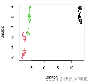
设置随机数为123，重新绘图：
代码为：

library(umap)
config.params = umap.defaults
config.params$random_state=123  ## 设置随机数
iris.umap <- umap(iris.data, config = config.params)
plot.data = as.data.frame(iris.umap$layout)
colnames(plot.data)=c("umap1","umap2")
head(plot.data)
plot(plot.data,col=as.factor(iris.labels), pch=20,cex=0.7)
1
2
3
4
5
6
7
8

上面参数修改方法在umap函数内也行；

iris.umap <- umap(iris.data, random_state=123) ## 直接函数内改变默认参数也可以
1

但有一点要注意，即便后面参数相同，如果输入的数据改变顺序，结果也会不同：
代码如下：

library(umap)
iris.data <- iris[, grep("Sepal|Petal", colnames(iris))]

## 增加重新排序，使原始数据顺序不同，结果也会不同
iris.data <- iris.data[order(iris.data$Sepal.Length),]

iris.labels <- iris[, "Species"]
config.params = umap.defaults
config.params$random_state=123
iris.umap <- umap(iris.data, random_state=123)
plot.data = as.data.frame(iris.umap$layout)
colnames(plot.data)=c("umap1","umap2")
plot(plot.data,col=as.factor(iris.labels), pch=20,cex=0.7)
1
2
3
4
5
6
7
8
9
10
11
12
13

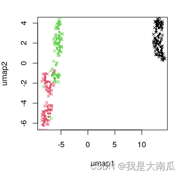
此外，可以进行波动数据映射到基础数据降维的umap结果中：

iris.data <- iris[, grep("Sepal|Petal", colnames(iris))]
iris.labels <- iris[, "Species"]

library(umap)
config.params = umap.defaults
config.params$random_state=123
iris.umap <- umap(iris.data, random_state=123)
plot.data = as.data.frame(iris.umap$layout)
colnames(plot.data)=c("umap1","umap2")
plot(plot.data,col=as.factor(iris.labels), pch=20,cex=0.7)


iris.wnoise <- iris.data + matrix(rnorm(150*40, 0, 0.1), ncol=4)
colnames(iris.wnoise) <- colnames(iris.data)
head(iris.wnoise, 3)
head(iris.data)
iris.wnoise.umap <- predict(iris.umap, iris.wnoise)
head(iris.wnoise.umap, 3)

points(iris.wnoise.umap, col=as.factor(iris.labels), pch=4,cex=0.7)
1
2
3
4
5
6
7
8
9
10
11
12
13
14
15
16
17
18
19
20

为保持结果的可重复性，umap结果需要设置随机种子，原始数据顺序也不能改变；
此外umap的输入数据可以为data，也可以是dist距离；
umap的knn也可以从已有的结果中提取，参考官方文档。

4. 总结

（1）PCA中（princomp和prcomp），推荐使用prcomp，使用范围更广；
（2）tSNE中（Rtsne和tsne）推荐Rtsne，参数更明确，可以选择pca模式（默认为pca模式），计算更快。二者均需要额外设定随机种子确保结果可重复；
（3）UMAP中参数设定可以通过外部参数设置，或者函数内设置，可以尝试更多参数，选择合适的结果。

总之，方法无好坏，数据特性不同，则适用不同方法。实际应用起来可能就需要多尝试了，结合实际问题选择。
本文也只是粗浅的过一遍，实际背后原理的这些，还得继续学习。

参考：
https://zhuanlan.zhihu.com/p/496823203 （PCA）
https://cloud.tencent.com/developer/article/1635055 （PCA）
https://stats.stackexchange.com/questions/268264/normalizing-all-the-variarbles-vs-using-scale-true-option-in-prcomp-in-r （PCA scale）
https://cloud.tencent.com/developer/article/1556202 （Rtsne）
https://stats.stackexchange.com/questions/222912/how-to-determine-parameters-for-t-sne-for-reducing-dimensions （Rtsne）
https://distill.pub/2016/misread-tsne/ （Rtsne parameters setting）
https://cran.r-project.org/web/packages/umap/vignettes/umap.html （R umap example）