多幅图像全景拼接代码修改

前言

参考代码：github代码地址

1、创建虚拟环境

conda create -n stitching python=3.7.0
1

2、激活虚拟环境

conda activate stitching
1

3、安装opencv和相应的包

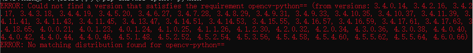
3.1 查看可安装opencv版本

相关opencv的最新版安装可见opencv安装

pip install opencv-python==
1

进行安装

pip install opencv-python==3.4.2.16
1

进行测试

3.2 安装对应的包

pip install imutils
1

3.3 安装opencv-contrib-python

出现报错

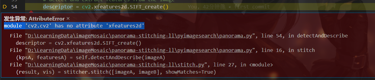
解决办法：补上一个版本配套的contrib包

pip install opencv-contrib-python==3.4.2.16
1

3.4 matplotlib安装

pip install matplotlib
1

3.5 PCV安装

可以参考PCV安装

1. 进入对应的文件夹clone PCV的代码

git clone https://github.com/Li-Shu14/PCV.git
1

2. 进行安装
   这里由于我是在windows环境安装的
   首先改变盘符到你对应的盘如D:
   进入文件夹cd xxx/PCV
   

python setup.py install
1

3.5 scipy安装

重新回到参考代码中，运行程序出现了报错

ModuleNotFoundError: No module named 'scipy'
1

在对应环境进行安装

pip install scipy
1

4、报错记录

4.1 print报错

SyntaxError: Missing parentheses in call to 'print'. Did you mean print('warp - right')?
1

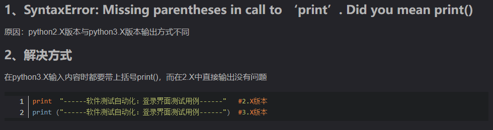
之前的PCV是应用于python2的，现在有针对python3更新的基于python3的PCVgithub

参考PCV安装基于python3进行安装

4.2 matplotlib.delaunay报错

ModuleNotFoundError: No module named 'matplotlib.delaunay'
1

更改方式可以参考matplotlib.delaunay报错
然后重新进行安装（这里不能直接进到对应的文件，所以修改完需要重新安装，我这里安装出现了报错，我直接删除了虚拟环境重新创建，然后进行安装）

4.3 无法生成.sift文件

  File "D:\anaconda\envs\stitching\lib\site-packages\numpy\lib\_datasource.py", line 533, in open
    raise IOError("%s not found." % path)
OSError: ./test/1027-1.sift not found.
1
2
3

参考链接：
OSError:sift not found 问题解决
图像拼接参考链接

1. VLfeat下载
   VLfeat下载
   

2. 选择对应的文件移入当前工程文件夹
   

3. 根据你自己的电脑是直接安装的Python还是Anaconda安装的找到对应目录中的【sift.py】文件
   直接安装的路径：python\Lib\site-packages\PCV\localdescriptors
   Anaconda安装的路径：Anaconda\Lib\site-packages\PCV\localdescriptors

4. 打开sift.py，修改路径
   打开【sift.py】文件，全局cmmd，将箭头指向的那个引号里的路径改为自己项目中【sift.exe】的路径
   注意：路径中如果用“\”则需要在前端加“r”，用’‘/’'或“\”则不需要
   
   
   成功生成sift文件

cmmd = str(r"D:/LearningData/imageMosaic/panoramic-image/sift.exe "+imagename+" --output="+resultname+ " "+params) 
1

4.4 图片差异太大

ValueError: did not meet fit acceptance criteria
1

多图拼接对图片的要求比较高，差异性大或太小（几乎相同）的拼接效果都很差。而且如果拍摄地点变动过大，会导致匹配值为0

5、拼接结果

5.1 两张图拼接

1. 原图
   
   

2. 获取特征
   

3. 拼接结果
   

5.2 两张不同角度图拼接

1. 原图
   
   

2. 特征
   

3. 结果
   
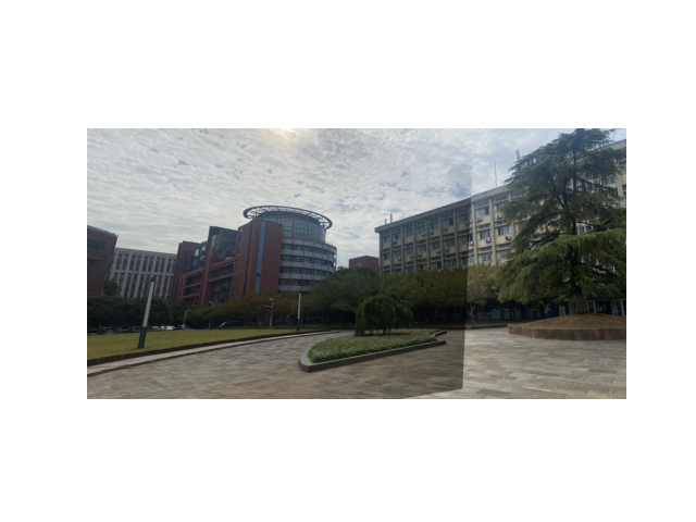
   景深有一定差异，但是对于不同角度的图像拼接还是可以进行拼接的

5.3 三张图拼接

1. 原图
   
   
   
   

2. 特征
   
   

3. 拼接结果
   

5.4 四图拼接

1. 原图
   
   
   
   

2. 特征图
   
   
   

3. 结果
   

对于多张图的拼接还是有些变形

5.5 五张图片拼接

1. 原图
   
   
   
   
   
   
   顺序自右向左

2. 特征
   
   
   
   

3. 结果
   

6、拼接过程梳理

1. 读取对应路径下的图片文件，提取特征保存在临时文件tmp.pgm中
   

2. 特征转换为对应的特征矩阵，保存在.sift文件中
   

3. 分别匹配临近两幅图的特征，可视化特征匹配

4. 通过封装的PCV方法与匹配到的特征求对应的变化矩阵、从而进行变换、扭曲、融合
   对应的变换矩阵如下
   

5. 可视化拼接结果
   

附录

1、PCV更改地址

基于4、5两个问题都是python版本导致的问题，修改后的代码我上传到了github
自己改的PCV代码

2、两幅图像拼接代码

from pylab import *
from numpy import *
from PIL import Image

# If you have PCV installed, these imports should work
from PCV.geometry import homography, warp
from PCV.localdescriptors import sift

"""
This is the panorama example from section 3.3.
"""

# set paths to data folder
# imname使我们要拼接的原图
# featname是sift文件，这个文件是需要根据原图进行生成的
# 需要根据自己的图像地址和图像数量修改地址和循环次数
# featname = ['./images5/'+str(i+1)+'.sift' for i in range(2)] 
# imname = ['./images5/'+str(i+1)+'.jpg' for i in range(2)]
featname = ['./test/1027-'+str(i+1)+'.sift' for i in range(2)] 
imname = ['./test/1027-'+str(i+1)+'.jpg' for i in range(2)]

# extract features and match
l = {}
d = {}
for i in range(2): 
    sift.process_image(imname[i],featname[i])
    l[i],d[i] = sift.read_features_from_file(featname[i])

matches = {}
for i in range(1):
    matches[i] = sift.match(d[i+1],d[i])

# visualize the matches (Figure 3-11 in the book)
for i in range(1):
    im1 = array(Image.open(imname[i]))
    im2 = array(Image.open(imname[i+1]))
    figure()
    sift.plot_matches(im2,im1,l[i+1],l[i],matches[i],show_below=True)


# function to convert the matches to hom. points
def convert_points(j):
    ndx = matches[j].nonzero()[0]
    fp = homography.make_homog(l[j+1][ndx,:2].T) 
    ndx2 = [int(matches[j][i]) for i in ndx]
    tp = homography.make_homog(l[j][ndx2,:2].T) 
    
    # switch x and y - TODO this should move elsewhere
    fp = vstack([fp[1],fp[0],fp[2]])
    tp = vstack([tp[1],tp[0],tp[2]])
    return fp,tp


# estimate the homographies
model = homography.RansacModel() 
# 此代码段为2图图像拼接，若需要多幅图，只需将其中的注释部分取消即可，图像顺序为自右向左。
fp,tp = convert_points(0)
H_01 = homography.H_from_ransac(fp,tp,model)[0] #im 0 to 1

#fp,tp = convert_points(1)
#H_12 = homography.H_from_ransac(fp,tp,model)[0] #im 1 to 2 

#tp,fp = convert_points(2) #NB: reverse order
#H_32 = homography.H_from_ransac(fp,tp,model)[0] #im 3 to 2 

#tp,fp = convert_points(3) #NB: reverse order
#H_43 = homography.H_from_ransac(fp,tp,model)[0] #im 4 to 3    


# warp the images
delta = 2000 # for padding and translation

im1 = array(Image.open(imname[0]), "uint8")
im2 = array(Image.open(imname[1]), "uint8")
im_12 = warp.panorama(H_01,im1,im2,delta,delta)
#im1 = array(Image.open(imname[0]), "f")
#im_02 = warp.panorama(dot(H_12,H_01),im1,im_12,delta,delta)

#im1 = array(Image.open(imname[3]), "f")
#im_32 = warp.panorama(H_32,im1,im_02,delta,delta)

#im1 = array(Image.open(imname[4]), "f")
#im_42 = warp.panorama(dot(H_32,H_43),im1,im_32,delta,2*delta)


figure()
imshow(array(im_12, "uint8"))
axis('off')
savefig("example1.png",dpi=300)
show()


1
2
3
4
5
6
7
8
9
10
11
12
13
14
15
16
17
18
19
20
21
22
23
24
25
26
27
28
29
30
31
32
33
34
35
36
37
38
39
40
41
42
43
44
45
46
47
48
49
50
51
52
53
54
55
56
57
58
59
60
61
62
63
64
65
66
67
68
69
70
71
72
73
74
75
76
77
78
79
80
81
82
83
84
85
86
87
88
89
90
91
92

3、三幅图像拼接代码

# 博客方法（三张图）
from pylab import *
from numpy import *
from PIL import Image
 
# If you have PCV installed, these imports should work
from PCV.geometry import homography, warp
from PCV.localdescriptors import sift
np.seterr(invalid='ignore') # 忽略部分警告
"""
This is the panorama example from section 3.3.
"""
 
# 设置数据文件夹的路径
featname = ['test/1027-'+str(i+1)+'.sift' for i in range(3)] 
imname = ['test/1027-'+str(i+1)+'.jpg' for i in range(3)]
 
# 提取特征并匹配使用sift算法
l = {}
d = {}
for i in range(3):
    sift.process_image(imname[i], featname[i]) # 处理图像并将结果保存到文件中tmp.pgm，进而保存到.sift文件中
    # feature locations, descriptors要素位置，描述符
    l[i], d[i] = sift.read_features_from_file(featname[i]) # 读取特征属性并以矩阵形式返回
# 特征间两两匹配
matches = {}
for i in range(2):
    matches[i] = sift.match(d[i + 1], d[i])
 
# 可视化匹配
for i in range(2):
    im1 = array(Image.open(imname[i]))
    im2 = array(Image.open(imname[i + 1]))
    figure()
    # im1、im2（图像作为数组）、locs1、locs2（特征位置）,matchscores（作为“match”的输出），show_below（如果下面应该显示图像）
    sift.plot_matches(im2, im1, l[i + 1], l[i], matches[i], show_below=True)
 
 
# 将匹配转换成齐次坐标点的函数
def convert_points(j):
    ndx = matches[j].nonzero()[0]
    fp = homography.make_homog(l[j + 1][ndx, :2].T)
    ndx2 = [int(matches[j][i]) for i in ndx]
    tp = homography.make_homog(l[j][ndx2, :2].T)
 
    # switch x and y - TODO this should move elsewhere
    fp = vstack([fp[1], fp[0], fp[2]])
    tp = vstack([tp[1], tp[0], tp[2]])
    return fp, tp
 
 
# 估计单应性矩阵
model = homography.RansacModel()
# 博客方法 
fp, tp = convert_points(1)
H_12 = homography.H_from_ransac(fp, tp, model)[0]  # im 1 to 2
print(H_12, 'H_12')
 
fp, tp = convert_points(0)
H_01 = homography.H_from_ransac(fp, tp, model)[0]  # im 0 to 1
print(H_01, 'H_01')
 
# tp, fp = convert_points(2)  # NB: reverse order
# H_32 = homography.H_from_ransac(fp, tp, model)[0]  # im 3 to 2
 
# tp, fp = convert_points(3)  # NB: reverse order
# H_43 = homography.H_from_ransac(fp, tp, model)[0]  # im 4 to 3


 
# 扭曲图像
delta = 1500  # for padding and translation用于填充和平移

# 博客方法
im1 = array(Image.open(imname[1]), "uint8")
im2 = array(Image.open(imname[2]), "uint8")
im_12 = warp.panorama(H_12, im1, im2, delta, delta)

im1 = array(Image.open(imname[0]), "f")
im_02 = warp.panorama(dot(H_12, H_01), im1, im_12, delta, delta)

# im1 = array(Image.open(imname[3]), "f")
# im_32 = warp.panorama(H_32, im1, im_02, delta, delta)

# im1 = array(Image.open(imname[4]), "f")
# im_42 = warp.panorama(dot(H_32, H_43), im1, im_32, delta, 2 * delta)


figure()
imshow(array(im_02, "uint8"))
axis('off')
show()
1
2
3
4
5
6
7
8
9
10
11
12
13
14
15
16
17
18
19
20
21
22
23
24
25
26
27
28
29
30
31
32
33
34
35
36
37
38
39
40
41
42
43
44
45
46
47
48
49
50
51
52
53
54
55
56
57
58
59
60
61
62
63
64
65
66
67
68
69
70
71
72
73
74
75
76
77
78
79
80
81
82
83
84
85
86
87
88
89
90
91
92

4、四幅图像拼接代码

from pylab import *
from numpy import *
from PIL import Image
 
# If you have PCV installed, these imports should work
from PCV.geometry import homography, warp
from PCV.localdescriptors import sift
np.seterr(invalid='ignore') # 忽略部分警告
"""
This is the panorama example from section 3.3.
"""
 
# 设置数据文件夹的路径
featname = ['test/1027-'+str(i+1)+'.sift' for i in range(4)] 
imname = ['test/1027-'+str(i+1)+'.jpg' for i in range(4)]
 
# 提取特征并匹配使用sift算法
l = {}
d = {}
for i in range(4):
    sift.process_image(imname[i], featname[i]) # 处理图像并将结果保存到文件中tmp.pgm，进而保存到.sift文件中
    # feature locations, descriptors要素位置，描述符
    l[i], d[i] = sift.read_features_from_file(featname[i]) # 读取特征属性并以矩阵形式返回
 
matches = {}
for i in range(3):
    matches[i] = sift.match(d[i + 1], d[i])
 
# 可视化匹配
for i in range(3):
    im1 = array(Image.open(imname[i]))
    im2 = array(Image.open(imname[i + 1]))
    figure()
    # im1、im2（图像作为数组）、locs1、locs2（特征位置）,matchscores（作为“match”的输出），show_below（如果下面应该显示图像）
    sift.plot_matches(im2, im1, l[i + 1], l[i], matches[i], show_below=True)
 
 
# 将匹配转换成齐次坐标点的函数
def convert_points(j):
    ndx = matches[j].nonzero()[0]
    fp = homography.make_homog(l[j + 1][ndx, :2].T)
    ndx2 = [int(matches[j][i]) for i in ndx]
    tp = homography.make_homog(l[j][ndx2, :2].T)
 
    # switch x and y - TODO this should move elsewhere
    fp = vstack([fp[1], fp[0], fp[2]])
    tp = vstack([tp[1], tp[0], tp[2]])
    return fp, tp
 
 
# 估计单应性矩阵
model = homography.RansacModel()
# 博客方法 
fp, tp = convert_points(1)
H_12 = homography.H_from_ransac(fp, tp, model)[0]  # im 1 to 2
 
fp, tp = convert_points(0)
H_01 = homography.H_from_ransac(fp, tp, model)[0]  # im 0 to 1
 
tp, fp = convert_points(2)  # NB: reverse order
H_32 = homography.H_from_ransac(fp, tp, model)[0]  # im 3 to 2
 
# tp, fp = convert_points(3)  # NB: reverse order
# H_43 = homography.H_from_ransac(fp, tp, model)[0]  # im 4 to 3

 
# 扭曲图像
delta = 2000  # for padding and translation用于填充和平移

# 博客方法
im1 = array(Image.open(imname[1]), "uint8")
im2 = array(Image.open(imname[2]), "uint8")
im_12 = warp.panorama(H_12, im1, im2, delta, delta)
 
im1 = array(Image.open(imname[0]), "f")
im_02 = warp.panorama(dot(H_12, H_01), im1, im_12, delta, delta)
 
im1 = array(Image.open(imname[3]), "f")
im_32 = warp.panorama(H_32, im1, im_02, delta, delta)
 
# im1 = array(Image.open(imname[4]), "f")
# im_42 = warp.panorama(dot(H_32, H_43), im1, im_32, delta, 2 * delta)



figure()
imshow(array(im_32, "uint8"))
axis('off')
show()
1
2
3
4
5
6
7
8
9
10
11
12
13
14
15
16
17
18
19
20
21
22
23
24
25
26
27
28
29
30
31
32
33
34
35
36
37
38
39
40
41
42
43
44
45
46
47
48
49
50
51
52
53
54
55
56
57
58
59
60
61
62
63
64
65
66
67
68
69
70
71
72
73
74
75
76
77
78
79
80
81
82
83
84
85
86
87
88
89

5、五张图像拼接代码

# -*- codeing =utf-8 -*-
# @Time : 2021/4/20 11:00
# @Author : ArLin
# @File : demo1.py
# @Software: PyCharm
from pylab import *
from numpy import *
from PIL import Image

# If you have PCV installed, these imports should work
from PCV.geometry import homography, warp
from PCV.localdescriptors import sift
np.seterr(invalid='ignore')
"""
This is the panorama example from section 3.3.
"""

# 设置数据文件夹的路径
featname = ['./test/1027-'+str(i+1)+'.sift' for i in range(5)] 
imname = ['./test/1027-'+str(i+1)+'.jpg' for i in range(5)]

# 提取特征并匹配使用sift算法
l = {}
d = {}
for i in range(5):
    sift.process_image(imname[i], featname[i])
    l[i], d[i] = sift.read_features_from_file(featname[i])

matches = {}
for i in range(4):
    matches[i] = sift.match(d[i + 1], d[i])

# 可视化匹配
for i in range(4):
    im1 = array(Image.open(imname[i]))
    im2 = array(Image.open(imname[i + 1]))
    figure()
    sift.plot_matches(im2, im1, l[i + 1], l[i], matches[i], show_below=True)


# 将匹配转换成齐次坐标点的函数
def convert_points(j):
    ndx = matches[j].nonzero()[0]
    fp = homography.make_homog(l[j + 1][ndx, :2].T)
    ndx2 = [int(matches[j][i]) for i in ndx]
    tp = homography.make_homog(l[j][ndx2, :2].T)

    # switch x and y - TODO this should move elsewhere
    fp = vstack([fp[1], fp[0], fp[2]])
    tp = vstack([tp[1], tp[0], tp[2]])
    return fp, tp


# 估计单应性矩阵
model = homography.RansacModel()

fp, tp = convert_points(1)
H_12 = homography.H_from_ransac(fp, tp, model)[0]  # im 1 to 2

fp, tp = convert_points(0)
H_01 = homography.H_from_ransac(fp, tp, model)[0]  # im 0 to 1

tp, fp = convert_points(2)  # NB: reverse order
H_32 = homography.H_from_ransac(fp, tp, model)[0]  # im 3 to 2

tp, fp = convert_points(3)  # NB: reverse order
H_43 = homography.H_from_ransac(fp, tp, model)[0]  # im 4 to 3

# 扭曲图像
delta = 2000  # for padding and translation用于填充和平移

im1 = array(Image.open(imname[1]), "uint8")
im2 = array(Image.open(imname[2]), "uint8")
im_12 = warp.panorama(H_12, im1, im2, delta, delta)

im1 = array(Image.open(imname[0]), "f")
im_02 = warp.panorama(dot(H_12, H_01), im1, im_12, delta, delta)

im1 = array(Image.open(imname[3]), "f")
im_32 = warp.panorama(H_32, im1, im_02, delta, delta)

im1 = array(Image.open(imname[4]), "f")
im_42 = warp.panorama(dot(H_32, H_43), im1, im_32, delta, 2 * delta)

figure()
imshow(array(im_42, "uint8"))
axis('off')
show()


1
2
3
4
5
6
7
8
9
10
11
12
13
14
15
16
17
18
19
20
21
22
23
24
25
26
27
28
29
30
31
32
33
34
35
36
37
38
39
40
41
42
43
44
45
46
47
48
49
50
51
52
53
54
55
56
57
58
59
60
61
62
63
64
65
66
67
68
69
70
71
72
73
74
75
76
77
78
79
80
81
82
83
84
85
86
87
88
89
90