Python优化算法02——遗传算法

参考文档链接：scikit-opt

---

本章继续Python的优化算法系列。

优化算法，尤其是启发式的仿生智能算法在最近很火，它适用于解决管理学，运筹学，统计学里面的一些优化问题。比如线性规划，整数规划，动态规划，非线性约束规划，甚至是超参数搜索等等方向的问题。

但是一般的优化算法还是matlab里面用的多，Python相关代码较少。博主在参考了很多文章的代码和模块之后，决定学习 scikit-opt   这个模块。这个优化算法模块对新手很友好，代码简洁，上手简单。而且代码和官方文档是中国人写的，还有很多案例，学起来就没什么压力...

缺点是包装的算法种类目前还不算多，只有七种：（差分进化算法、遗传算法、粒子群算法、模拟退火算法、蚁群算法、鱼群算法、免疫优化算法）      /（其实已经够用了）

本次带来的是 数学建模里面经常使用的遗传算法的使用演示。数学原理就不多说了

---

首先安装模块，在cmd里面或者anaconda prompt里面输入：

pip install scikit-opt

这个包很小，很快就能装好。

---

遗传算法

首先定义我们要解决的优化的问题：

 

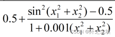
该函数有大量的局部最小值，具有很强的冲击力，在(0,0) 处的全局最小值，值为 0

代码

import numpy as np
 
def schaffer(p):
    x1, x2 = p
    x = np.square(x1) + np.square(x2)
    return 0.5 + (np.square(np.sin(x)) - 0.5) / np.square(1 + 0.001 * x)

调用遗传算法GA解决：

from sko.GA import GA
 
ga = GA(func=schaffer, n_dim=2, size_pop=50, max_iter=800, prob_mut=0.001, lb=[-1, -1], ub=[1, 1], precision=1e-7)
best_x, best_y = ga.run()
print('best_x:', best_x, '\n', 'best_y:', best_y)

可以看到基本找到了全局最小值和对应的x 。

画出迭代次数的图

import pandas as pd
import matplotlib.pyplot as plt
 
Y_history = pd.DataFrame(ga.all_history_Y)
fig, ax = plt.subplots(2, 1)
ax[0].plot(Y_history.index, Y_history.values, '.', color='red')
Y_history.min(axis=1).cummin().plot(kind='line')
plt.show()

---

参数详解

上面用到了很多参数，不懂可以看看这里

输入参数

 输出参数

---

遗传算法进行整数规划

在多维优化时，想让哪个变量限制为整数，就设定 precision 为 整数 即可。
例如，我想让我的自定义函数 demo_func 的某些变量限制为整数+浮点数（分别是整数，整数，浮点数），那么就设定 precision=[1, 1, 1e-7]
例子如下：

from sko.GA import GA
 
demo_func = lambda x: (x[0] - 1) ** 2 + (x[1] - 0.05) ** 2 + x[2] ** 2
 
ga = GA(func=demo_func, n_dim=3, max_iter=500, lb=[-1, -1, -1], ub=[5, 1, 1], precision=[1,1,1e-7])
best_x, best_y = ga.run()
print('best_x:', best_x, '\n', 'best_y:', best_y)

可以看到第一个、第二个变量都是整数，第三个就是浮点数了 。

---

遗传算法用于旅行商问题

商旅问题(TSP)就是路径规划的问题，比如有很多城市，你都要跑一遍，那么先去哪个城市再去哪个城市可以让你的总路程最小。

实际问题需要一个城市坐标数据，比如你的出发点位置为（0,0），第一个城市离位置为（x1,y1）,第二个为（x2,y2）.........这里没有实际数据，就直接随机生成了。

import numpy as np
from scipy import spatial
import matplotlib.pyplot as plt
 
num_points = 50
points_coordinate = np.random.rand(num_points, 2)  # generate coordinate of points
points_coordinate 

 

 这里定义的是50个城市，每个城市的坐标都在是上图随机生成的矩阵。

然后我们把它变成类似相关系数里面的矩阵

distance_matrix = spatial.distance.cdist(points_coordinate, points_coordinate, metric='euclidean')
distance_matrix.shape

 这个矩阵就能得出每个城市之间的距离，算上自己和自己的距离（0），总共有2500个数。

定义问题

def cal_total_distance(routine):
    num_points, = routine.shape
    return sum([distance_matrix[routine[i % num_points], routine[(i + 1) % num_points]] for i in range(num_points)])

求解

from sko.GA import GA_TSP
ga_tsp = GA_TSP(func=cal_total_distance, n_dim=num_points, size_pop=50, max_iter=500, prob_mut=1)
best_points, best_distance = ga_tsp.run()

best_distance

得到的最小距离

画图查看计算出来的路径，还有迭代次数和y的关系

fig, ax = plt.subplots(1, 2,figsize=(10,4))
best_points_ = np.concatenate([best_points, [best_points[0]]])
best_points_coordinate = points_coordinate[best_points_, :]
ax[0].plot(best_points_coordinate[:, 0], best_points_coordinate[:, 1], 'o-r')
ax[1].plot(ga_tsp.generation_best_Y)
plt.show()

 

---

使用遗传算法进行曲线拟合

构建数据集

import numpy as np
import matplotlib.pyplot as plt
from sko.GA import GA
 
x_true = np.linspace(-1.2, 1.2, 30)
y_true = x_true ** 3 - x_true + 0.4 * np.random.rand(30)
plt.plot(x_true, y_true, 'o')

构建的数据是y=x^3-x+0.4,然后加上了随机扰动项。如图

 定义需要拟合的函数（三次函数），然后将残差作为目标函数去求解

def f_fun(x, a, b, c, d):
    return a * x ** 3 + b * x ** 2 + c * x + d   #三次函数
 
def obj_fun(p):
    a, b, c, d = p
    residuals = np.square(f_fun(x_true, a, b, c, d) - y_true).sum()
    return residuals

求解 

ga = GA(func=obj_fun, n_dim=4, size_pop=100, max_iter=500,
        lb=[-2] * 4, ub=[2] * 4)
 
best_params, residuals = ga.run()
print('best_x:', best_params, '\n', 'best_y:', residuals)

可以看到拟合出来的方程为y=0.919x^3-0.0244x^2-0.939x+0.2152.

拟合效果还行 

 画出拟合线

y_predict = f_fun(x_true, *best_params)
 
fig, ax = plt.subplots()
ax.plot(x_true, y_true, 'o')
ax.plot(x_true, y_predict, '-')
 
plt.show()