-
猿创征文|数据导入与预处理-第3章-pandas基础
猿创征文|数据导入与预处理-第3章-pandas基础
1 Pandas概述
1.1 pandas官网阅读指南
pandas的官网地址为:https://pandas.pydata.org/
官网首页介绍了Pandas,pandas is a fast, powerful, flexible and easy to use open source data analysis and manipulation tool,
built on top of the Python programming language.
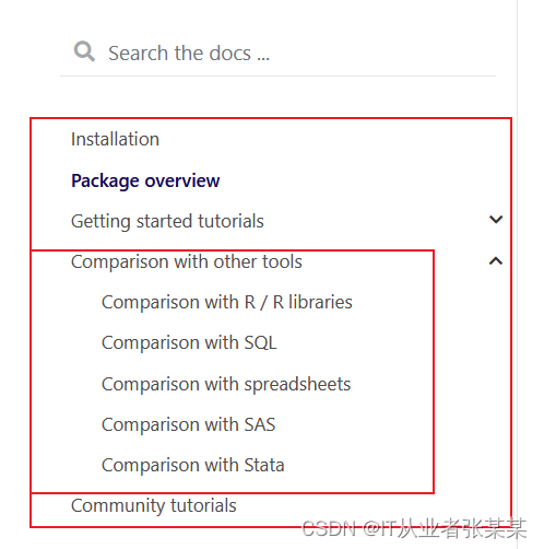
pandas是一个快速、强大、灵活且易于使用的开源数据分析和操作工具,构建在Python编程语言之上。点击导航栏中的document,再点击getting started,会进入到pandas对应的文档页。地址如下:https://pandas.pydata.org/docs/getting_started/index.html#getting-started
通过右面的英文菜单,可以辅助我们更好的理解pandas是什么
在对pandas有了基本了解后,就可以通过用户指南进行pandas的练习了。关于pandas,官方的解释是,pandas是一个基于BSD开源协议的开源库,提供了用于python编程语言的高性能、易于使用的数据结构和数据分析工具。
这里还提到了BSD开源协议。BSD开源协议可以自修改源代码,也可以将修改后的代码作为开源或者专有软件再发布。
但需要满足三个条件:
1.如果再发布的产品中包含源代码,则在源代码中必须带有原来代码中的BSD协议。
2.如果再发布的只是二进制类库/软件,则需要在类库/软件的文档和版权声明中包含原来代码中的BSD协议。
3.不可以用开源代码的作者/机构名字和原来产品的名字做市场推广。1.2 Pandas中的数据结构
对于pandas这种数据分析库而已,我们都可以通过与传统的集合对象来理解,pandas提供了类似集合的数据结构,也提供了对应属性和方法,我们只需要把数据封装到pandas提供的数据结构对象中,既可以使用pandas库提供的实用的高效的方法。
pandas提供了2种常见的数据结构,分别为:Series、DataFrame。
Series是用于处理一维数据的;dataframe则是处理二维数据的。1.3 Series
1.3.1 Series简介
Series是一个结构类似于一维数组的对象,该对象主要由索引数据和索引两部分组成,其中数据可以是任意类型,比如整数、字符串、浮点数等。
Series类对象的索引样式比较丰富,默认是自动生成的整数索引(从0开始递增),也可以是自定义的标签索引(由自定义的标签构成的索引)、时间戳索引(由时间戳构成的索引)等。如下所示:
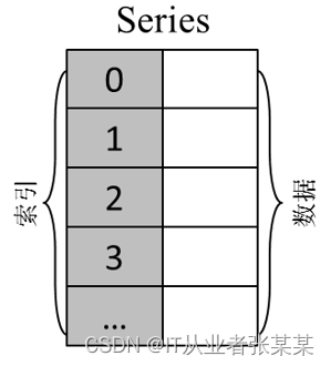
左侧的灰色轴表示标签轴,也就是index轴索引,在标签为"0""1""2"和"3"的后面存放的是对应的数据。
通过Series类的构造方法可以创建一维数据:pandas.Series(data=None,index=None,dtype=None, name=None,copy=False, fastpath=False)- 1
- 2
data:表示传入的数据,可以是ndarry、list、dict等。
index:表示传入的索引,必须是唯一的,且与数据的长度相同。若没有传入索引,则创建的Series类对象会自动生成0~N的整数索引。
dtype:表示数据的类型。若未指定数据类型,pandas会根据传入的数据自动推断数据类型。
在使用pandas中的Series数据结构时,可通过pandas点Series调用。有时,这样写有些麻烦,这时,可单独引入Series数据结构,通过代码“from空格pandas空格important空格Series”实现,当然,这里也可以使用“AS”设置别名。这样就不需要每次都写“pandas点Series”,简单又方便。from pandas import Series [as 别名]。- 1
1.3.2创建Series对象:
- 基于列表创建:
In [1]: import pandas as pd In [2]: ser_obj = pd.Series(['Python', 'Java', 'PHP']) In [3]: ser_obj- 1
- 2
- 3
输出为:
Out[3]:
0 Python
1 Java
2 PHP
dtype: object- 基于字典创建
In [3]: data = {'one': 'Python', 'two': 'Java','three': 'PHP'} In [4]: ser_obj2 = pd.Series(data) In [5]: ser_obj2- 1
- 2
- 3
输出为:
Out[5]:
one Python
two Java
three PHP
dtype: object- 创建Series类的对象并指定索引
import pandas as pd ser_obj = pd.Series(['Python', 'Java', 'PHP'], index = ['one', 'two', 'three']) ser_obj- 1
- 2
- 3
输出为:
Out[4]:
one Python
two Java
three PHP
dtype: object- 由数组创建(一维数组)
import numpy as np import pandas as pd arr = np.random.randn(5) s = pd.Series(arr) # 默认index是从0开始,步长为1的数字 s = pd.Series(arr, index = ['a','b','c','d','e'],dtype = np.object) s- 1
- 2
- 3
- 4
- 5
- 6
- 7
输出为:
Out[9]:
a 3.49113
b -0.206911
c -0.94533
d -0.818286
e -0.634007
dtype: object- 由标量创建
In [10]: s = pd.Series(10, index = range(4)) ...: s ...:- 1
- 2
- 3
- 4
输出为:
Out[10]:
0 10
1 10
2 10
3 10
dtype: int64思考:如果传入的数据对象类型不一致怎样办?
1.3.3Series属性
- Series的index和values属性
In [5]: print(ser_obj.index,type(ser_obj.index)) Index(['one', 'two', 'three'], dtype='object') <class 'pandas.core.indexes.base.Index'> In [6]: print(ser_obj.values,type(ser_obj.values)) ['Python' 'Java' 'PHP'] <class 'numpy.ndarray'>- 1
- 2
- 3
- 4
- 5
从结果可以看出:
核心:series相比于ndarray,是一个自带索引index的数组 → 一维数组 + 对应索引
所以当只看series的值的时候,就是一个ndarray
series和ndarray较相似,索引切片功能差别不大
series和dict相比,series更像一个有顺序的字典(dict本身不存在顺序),其索引原理与字典相似(一个用key,一个用index)- Series的name属性
# Series 名称属性:name s1 = pd.Series(np.random.randn(5)) s1- 1
- 2
- 3
输出为:
Out[11]:
0 0.820317
1 -0.260753
2 -0.512390
3 -0.782781
4 0.977223
dtype: float64s2 = pd.Series(np.random.randn(5),name = 'test') s2- 1
- 2
输出为:
Out[12]:
0 -2.690275
1 0.346298
2 -0.223346
3 -1.203251
4 0.374382
Name: test, dtype: float64In [13]: print(s1.name, s2.name,type(s2.name))- 1
输出为:
None test
# name为Series的一个参数,创建一个数组的名称 # .name方法:输出数组的名称,输出格式为str,如果没用定义输出名称,输出为None s3 = s2.rename('hehehe') s3- 1
- 2
- 3
- 4
输出为:
Out[15]:
0 -2.690275
1 0.346298
2 -0.223346
3 -1.203251
4 0.374382
Name: hehehe, dtype: float64print(s3.name, s2.name) # .rename()重命名一个数组的名称,并且新指向一个数组,原数组不变- 1
输出为:
hehehe test
1.3.4 Series索引
包括:位置下标 / 标签索引 / 切片索引 / 布尔型索引
- 位置索引
# 位置下标,类似序列 s = pd.Series(np.random.rand(5)) s- 1
- 2
- 3
输出为:
Out[18]:
0 0.453055
1 0.208872
2 0.917167
3 0.238751
4 0.720561
dtype: float64In [19]: print(s[0],type(s[0]),s[0].dtype)- 1
输出为:
0.45305476973470404
float64 In [20]: print(float(s[0]),type(float(s[0])))- 1
输出为:
0.45305476973470404
位置下标从0开始,输出结果为numpy.float格式,可以通过float()函数转换为python float格式,numpy.float与float占用字节不同,s[-1]会报错?
- 标签索引
# 标签索引 s = pd.Series(np.random.rand(5), index = ['a','b','c','d','e']) s- 1
- 2
- 3
输出为:
Out[22]:
a 0.037435
b 0.536072
c 0.051238
d 0.906477
e 0.474856
dtype: float64print(s['a'],type(s['a']),s['a'].dtype) # 方法类似下标索引,用[]表示,内写上index,注意index是字符串- 1
- 2
输出为:
0.037435262125128266
float64 sci = s[['a','b','e']] print(sci,type(sci)) # 如果需要选择多个标签的值,用[[]]来表示(相当于[]中包含一个列表) # 多标签索引结果是新的数组- 1
- 2
- 3
- 4
输出为:
a 0.037435
b 0.536072
e 0.474856
dtype: float64- 切片索引
# 切片索引 s1 = pd.Series(np.random.rand(5)) s2 = pd.Series(np.random.rand(5), index = ['a','b','c','d','e']) print('-----') print(s1[1:4],s1[4]) print(s2['a':'c'],s2['c']) print(s2[0:3],s2[3]) print('-----') # 注意:用index做切片是末端包含 print(s2[:-1]) print(s2[::2]) # 下标索引做切片,和list写法一样- 1
- 2
- 3
- 4
- 5
- 6
- 7
- 8
- 9
- 10
- 11
- 12
- 13
输出为:
-----
1 0.792143
2 0.876208
3 0.542396
dtype: float64 0.3478167781738142
a 0.338142
b 0.314807
c 0.716646
dtype: float64 0.7166457177011984
a 0.338142
b 0.314807
c 0.716646
dtype: float64 0.7435841750851758
-----
a 0.338142
b 0.314807
c 0.716646
d 0.743584
dtype: float64
a 0.338142
c 0.716646
e 0.499374
dtype: float64- 布尔索引
s = pd.Series(np.random.rand(3)*100) s[4] = None # 添加一个空值 s- 1
- 2
- 3
输出为:
Out[28]:
0 10.7214
1 72.9608
2 23.8594
4 None
dtype: objectbs1 = s > 50 bs2 = s.isnull() bs3 = s.notnull() print('-----') print(bs1, type(bs1), bs1.dtype) print(bs2, type(bs2), bs2.dtype) print(bs3, type(bs3), bs3.dtype) print('-----')- 1
- 2
- 3
- 4
- 5
- 6
- 7
- 8
输出为:
-----
0 False
1 True
2 False
4 False
dtype: boolbool
0 False
1 False
2 False
4 True
dtype: boolbool
0 True
1 True
2 True
4 False
dtype: boolbool
-----# 数组做判断之后,返回的是一个由布尔值组成的新的数组 # .isnull() / .notnull() 判断是否为空值 (None代表空值,NaN代表有问题的数值,两个都会识别为空值) s[s > 50]- 1
- 2
- 3
输出为:
Out[32]:
1 72.9608
dtype: objects[bs3] # 布尔型索引方法:用[判断条件]表示,其中判断条件可以是 一个语句,或者是 一个布尔型数组!- 1
- 2
输出为:
Out[33]:
0 10.7214
1 72.9608
2 23.8594
dtype: object1.3.5 Series基本操作技巧
本部分主要包括数据查看 / 重新索引 / 对齐 / 添加、修改、删除值等。
- 数据查看:
# 数据查看 s = pd.Series(np.random.rand(50)) # s.head(10) s.tail()- 1
- 2
- 3
- 4
输出为:
Out[34]:
45 0.805533
46 0.050284
47 0.423695
48 0.939936
49 0.124114
dtype: float64- 重新索引
# 重新索引reindex # .reindex将会根据索引重新排序,如果当前索引不存在,则引入缺失值 s = pd.Series(np.random.rand(3), index = ['a','b','c']) s- 1
- 2
- 3
- 4
输出为:
Out[35]:
a 0.062014
b 0.735581
c 0.730702
dtype: float64s1 = s.reindex(['c','b','a','d']) s1 # .reindex()中也是写列表 # 这里'd'索引不存在,所以值为NaN- 1
- 2
- 3
- 4
输出为:
Out[36]:
c 0.730702
b 0.735581
a 0.062014
d NaN
dtype: float64s2 = s.reindex(['c','b','a','d'], fill_value = 0) s2 # fill_value参数:填充缺失值的值- 1
- 2
- 3
输出为:
Out[37]:
c 0.730702
b 0.735581
a 0.062014
d 0.000000
dtype: float64- 数据对齐
# Series对齐 s1 = pd.Series(np.random.rand(3), index = ['Jack','Marry','Tom']) s2 = pd.Series(np.random.rand(3), index = ['Wang','Jack','Marry']) print('s1:',s1) print('s2:',s2)- 1
- 2
- 3
- 4
- 5
输出为:
s1:
Jack 0.733634
Marry 0.996989
Tom 0.951236
dtype: float64
s2:
Wang 0.931015
Jack 0.220763
Marry 0.391837
dtype: float64s1 + s2- 1
输出为:
Out[41]:
Jack 0.954397
Marry 1.388826
Tom NaN
Wang NaN
dtype: float64Series 和 ndarray 之间的主要区别是,Series 上的操作会根据标签自动对齐
index顺序不会影响数值计算,以标签来计算
空值和任何值计算结果扔为空值- 数据删除
In [44]: # 删除:.drop s = pd.Series(np.random.rand(5), index = list('ngjur')) s- 1
- 2
- 3
- 4
输出为:
Out[44]:
n 0.820846
g 0.825120
j 0.881528
u 0.321654
r 0.560360
dtype: float64In [45]: s1 = s.drop('n') s1- 1
- 2
- 3
输出为:
Out[45]: g 0.825120 j 0.881528 u 0.321654 r 0.560360 dtype: float64- 1
- 2
- 3
- 4
- 5
- 6
In [46]: s2 = s.drop(['g','j']) s2- 1
- 2
- 3
输出为:
Out[46]:
n 0.820846
u 0.321654
r 0.560360
dtype: float64In [47]: s # drop 删除元素之后返回副本(inplace=False)- 1
- 2
- 3
输出为:
Out[47]:
n 0.820846
g 0.825120
j 0.881528
u 0.321654
r 0.560360
dtype: float64- 添加
In [49]: # 添加 s1 = pd.Series(np.random.rand(5)) s1- 1
- 2
- 3
- 4
输出为:
Out[49]:
0 0.549820
1 0.563056
2 0.195393
3 0.348328
4 0.382846
dtype: float64In [50]: s2 = pd.Series(np.random.rand(5), index = list('ngjur')) s2- 1
- 2
- 3
输出为:
Out[50]:
n 0.381726
g 0.842261
j 0.878494
u 0.093220
r 0.604935
dtype: float64In [51]: s1[5] = 100 s1- 1
- 2
- 3
输出为:
Out[51]:
0 0.549820
1 0.563056
2 0.195393
3 0.348328
4 0.382846
5 100.000000
dtype: float64In [52]: s2['a'] = 100 s2- 1
- 2
- 3
输出为:
Out[52]:
n 0.381726
g 0.842261
j 0.878494
u 0.093220
r 0.604935
a 100.000000
dtype: float64In [54]: # 直接通过下标索引/标签index添加值 s3 = s1.append(s2) s3- 1
- 2
- 3
- 4
输出为:
Out[54]:
0 0.549820
1 0.563056
2 0.195393
3 0.348328
4 0.382846
5 100.000000
n 0.381726
g 0.842261
j 0.878494
u 0.093220
r 0.604935
a 100.000000
dtype: float64In [55]: s1 # 通过.append方法,直接添加一个数组 # .append方法生成一个新的数组,不改变之前的数组- 1
- 2
- 3
- 4
输出为:
Out[55]:
0 0.549820
1 0.563056
2 0.195393
3 0.348328
4 0.382846
5 100.000000
dtype: float64- 数据修改
In [57]: # 修改 s = pd.Series(np.random.rand(3), index = ['a','b','c']) s- 1
- 2
- 3
- 4
- 5
输出为:
Out[57]:
a 0.933075
b 0.861651
c 0.042825
dtype: float64In [58]: s['a'] = 100 s[['b','c']] = 200 s # 通过索引直接修改,类似序列- 1
- 2
- 3
- 4
- 5
输出为:
Out[58]:
a 100.0
b 200.0
c 200.0
dtype: float641.4 DataFrame
1.4.1 Dataframe简介
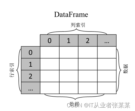
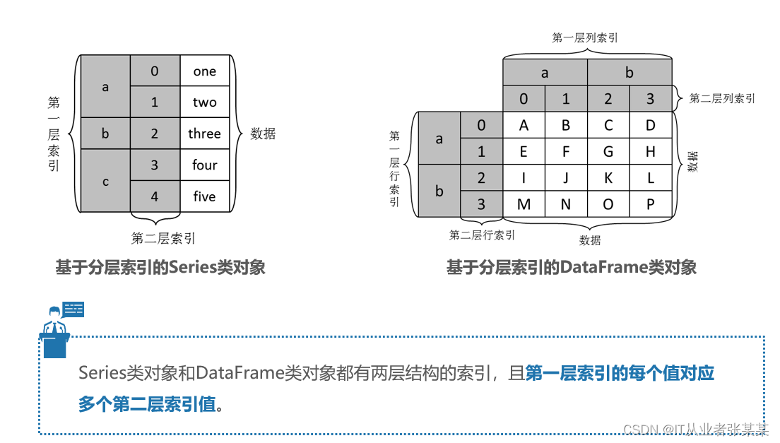
DataFrame是一个结构类似于二维数组或表格的对象,与Series类对象相比,DataFrame类对象也由索引和数据组成,但该对象有两组索引,分别是行索引和列索引。
DataFrame类对象的行索引位于最左侧一列,列索引位于最上面一行,且每个列索引对应着一列数据。DataFrame类对象其实可以视为若干个公用行索引的Series类对象的组合。如下所示:
"二维数组"Dataframe:是一个表格型的数据结构,包含一组有序的列,其列的值类型可以是数值、字符串、布尔值等。
Dataframe中的数据以一个或多个二维块存放,不是列表、字典或一维数组结构。通过DataFrame()类的构造方法可以创建二维数据
pandas.DataFrame(data=None, index=None, columns=None, dtype=None, copy=False)- 1
- 2
data:表示传入的数据,可以是ndarray、dict、list或可迭代对象。
index:表示行索引,默认生成0~N的整数索引。
columns:表示列索引,默认生成0~N的整数索引。
dtype:表示数据的类型。1.4.2 创建DataFrame对象
- 创建DataFrame类的对象,通过ndarray
In [29]: demo_arr = np.array([['a', 'b', 'c'],['d', 'e', 'f']]) df_obj = pd.DataFrame(demo_arr) df_obj- 1
- 2
- 3
- 4
输出为:
Out[29]:
0 1 2
0 a b c
1 d e f- 创建DataFrame类的对象并指定索引
In [31]: df_obj = pd.DataFrame(demo_arr,index = ['row_01','row_02'],columns=['col_01', 'col_02', 'col_03']) df_obj- 1
- 2
- 3
输出为:
Out[31]:
col_01 col_02 col_03
row_01 a b c
row_02 d e f可以测试下如何index的数量和行数不一致,会发生什么?
- 创建DataFrame类的对象,基于字典
import pandas as pd import numpy as np # Dataframe 数据结构 # Dataframe是一个表格型的数据结构,“带有标签的二维数组”。 # Dataframe带有index(行标签)和columns(列标签) data = {'name':['Jack','Tom','Mary'], 'age':[18,19,20], 'gender':['m','m','w']} frame = pd.DataFrame(data) print(frame) print(type(frame)) print(frame.index,'\n该数据类型为:',type(frame.index)) print(frame.columns,'\n该数据类型为:',type(frame.columns)) print(frame.values,'\n该数据类型为:',type(frame.values)) # 查看数据,数据类型为dataframe # .index查看行标签 # .columns查看列标签 # .values查看值,数据类型为ndarray- 1
- 2
- 3
- 4
- 5
- 6
- 7
- 8
- 9
- 10
- 11
- 12
- 13
- 14
- 15
- 16
- 17
- 18
- 19
输出为:
name age gender
0 Jack 18 m
1 Tom 19 m
2 Mary 20 w
RangeIndex(start=0, stop=3, step=1)
该数据类型为:
Index([‘name’, ‘age’, ‘gender’], dtype=‘object’)
该数据类型为:
[[‘Jack’ 18 ‘m’]
[‘Tom’ 19 ‘m’]
[‘Mary’ 20 ‘w’]]
该数据类型为:- 创建DataFrame类的对象,由Series组成的字典
# Dataframe 创建方法二:由Series组成的字典 data1 = {'one':pd.Series(np.random.rand(2)), 'two':pd.Series(np.random.rand(3))} # 没有设置index的Series data2 = {'one':pd.Series(np.random.rand(2), index = ['a','b']), 'two':pd.Series(np.random.rand(3),index = ['a','b','c'])} # 设置了index的Series print(data1) print(data2) df1 = pd.DataFrame(data1) df2 = pd.DataFrame(data2) print(df1) print(df2) # 由Seris组成的字典 创建Dataframe,columns为字典key,index为Series的标签(如果Series没有指定标签,则是默认数字标签) # Series可以长度不一样,生成的Dataframe会出现NaN值- 1
- 2
- 3
- 4
- 5
- 6
- 7
- 8
- 9
- 10
- 11
- 12
- 13
- 14
输出为:
{‘one’: 0 0.089832
1 0.519983
dtype: float64, ‘two’: 0 0.449765
1 0.036004
2 0.708951
dtype: float64}
{‘one’: a 0.607911
b 0.320829
dtype: float64, ‘two’: a 0.413806
b 0.871358
c 0.529347
dtype: float64}
one two
0 0.089832 0.449765
1 0.519983 0.036004
2 NaN 0.708951
one two
a 0.607911 0.413806
b 0.320829 0.871358
c NaN 0.529347- 创建DataFrame类的对象,由字典组成的字典
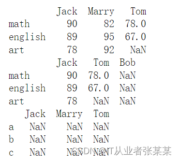
# Dataframe 创建方法五:由字典组成的字典 data = {'Jack':{'math':90,'english':89,'art':78}, 'Marry':{'math':82,'english':95,'art':92}, 'Tom':{'math':78,'english':67}} df1 = pd.DataFrame(data) print(df1) # 由字典组成的字典创建Dataframe,columns为字典的key,index为子字典的key df2 = pd.DataFrame(data, columns = ['Jack','Tom','Bob']) df3 = pd.DataFrame(data, index = ['a','b','c']) print(df2) print(df3) # columns参数可以增加和减少现有列,如出现新的列,值为NaN # index在这里和之前不同,并不能改变原有index,如果指向新的标签,值为NaN (非常重要!)- 1
- 2
- 3
- 4
- 5
- 6
- 7
- 8
- 9
- 10
- 11
- 12
- 13
- 14
- 15
输出为:
1.4.3 Dataframe:索引
Dataframe既有行索引也有列索引,可以被看做由Series组成的字典(共用一个索引)
选择列 / 选择行 / 切片 / 布尔判断- 选择行与列
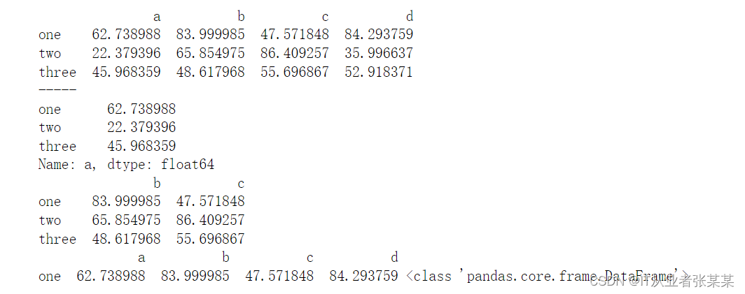
# 选择行与列 df = pd.DataFrame(np.random.rand(12).reshape(3,4)*100, index = ['one','two','three'], columns = ['a','b','c','d']) print(df) data1 = df['a'] data2 = df[['a','c']] print(data1,type(data1)) print(data2,type(data2)) print('-----') # 按照列名选择列,只选择一列输出Series,选择多列输出Dataframe data3 = df.loc['one'] data4 = df.loc[['one','two']] print(data2,type(data3)) print(data3,type(data4)) # 按照index选择行,只选择一行输出Series,选择多行输出Dataframe- 1
- 2
- 3
- 4
- 5
- 6
- 7
- 8
- 9
- 10
- 11
- 12
- 13
- 14
- 15
- 16
- 17
- 18
输出为:
 df[] - 选择列
一般用于选择列,也可以选择行- df[] - 选择行
# df[] - 选择列 # 一般用于选择列,也可以选择行 df = pd.DataFrame(np.random.rand(12).reshape(3,4)*100, index = ['one','two','three'], columns = ['a','b','c','d']) print(df) print('-----') data1 = df['a'] data2 = df[['b','c']] # 尝试输入 data2 = df[['b','c','e']] print(data1) print(data2) # df[]默认选择列,[]中写列名(所以一般数据colunms都会单独制定,不会用默认数字列名,以免和index冲突) # 单选列为Series,print结果为Series格式 # 多选列为Dataframe,print结果为Dataframe格式 data3 = df[:1] #data3 = df[0] #data3 = df['one'] print(data3,type(data3)) # df[]中为数字时,默认选择行,且只能进行切片的选择,不能单独选择(df[0]) # 输出结果为Dataframe,即便只选择一行 # df[]不能通过索引标签名来选择行(df['one']) # 核心笔记:df[col]一般用于选择列,[]中写列名- 1
- 2
- 3
- 4
- 5
- 6
- 7
- 8
- 9
- 10
- 11
- 12
- 13
- 14
- 15
- 16
- 17
- 18
- 19
- 20
- 21
- 22
- 23
- 24
- 25
- 26
输出为:
- df.loc[] - 按index选择行
# df.loc[] - 按index选择行 df1 = pd.DataFrame(np.random.rand(16).reshape(4,4)*100, index = ['one','two','three','four'], columns = ['a','b','c','d']) df2 = pd.DataFrame(np.random.rand(16).reshape(4,4)*100, columns = ['a','b','c','d']) print(df1) print(df2) print('-----') data1 = df1.loc['one'] data2 = df2.loc[1] print(data1) print(data2) print('单标签索引\n-----') # 单个标签索引,返回Series # data3 = df1.loc[['two','three','five']] #不再支持不存在的index,本例为'five' data4 = df2.loc[[3,2,1]] #print(data3) print(data4) print('多标签索引\n-----') # 多个标签索引,如果标签不存在,则返回NaN # 顺序可变 data5 = df1.loc['one':'three'] data6 = df2.loc[1:3] print(data5) print(data6) print('切片索引') # 可以做切片对象 # 末端包含 # 核心笔记:df.loc[label]主要针对index选择行,同时支持指定index,及默认数字index- 1
- 2
- 3
- 4
- 5
- 6
- 7
- 8
- 9
- 10
- 11
- 12
- 13
- 14
- 15
- 16
- 17
- 18
- 19
- 20
- 21
- 22
- 23
- 24
- 25
- 26
- 27
- 28
- 29
- 30
- 31
- 32
- 33
- 34
- 35
输出为:

- df.iloc[] - 按照整数位置(从轴的0到length-1)选择行
# df.iloc[] - 按照整数位置(从轴的0到length-1)选择行 # 类似list的索引,其顺序就是dataframe的整数位置,从0开始计 df = pd.DataFrame(np.random.rand(16).reshape(4,4)*100, index = ['one','two','three','four'], columns = ['a','b','c','d']) print(df) print('------') print(df.iloc[0]) print(df.iloc[-1]) #print(df.iloc[4]) print('单位置索引\n-----') # 单位置索引 # 和loc索引不同,不能索引超出数据行数的整数位置 print(df.iloc[[0,2]]) print(df.iloc[[3,2,1]]) print('多位置索引\n-----') # 多位置索引 # 顺序可变 print(df.iloc[1:3]) print(df.iloc[::2]) print('切片索引') # 切片索引 # 末端不包含- 1
- 2
- 3
- 4
- 5
- 6
- 7
- 8
- 9
- 10
- 11
- 12
- 13
- 14
- 15
- 16
- 17
- 18
- 19
- 20
- 21
- 22
- 23
- 24
- 25
- 26
- 27
输出为:

- 布尔型索引
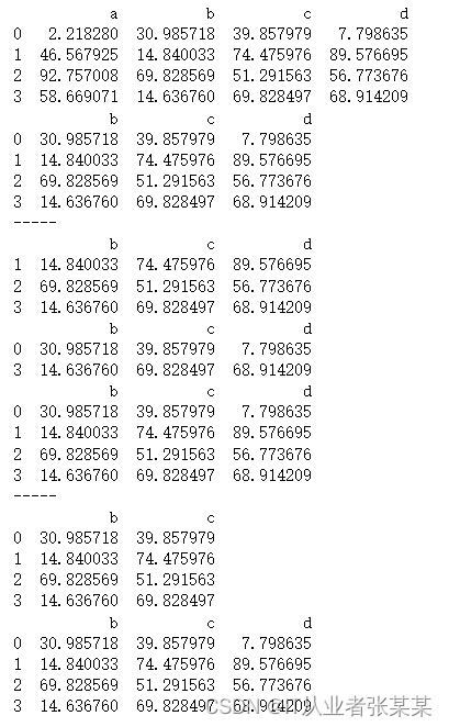
# 布尔型索引 # 和Series原理相同 df = pd.DataFrame(np.random.rand(16).reshape(4,4)*100, index = ['one','two','three','four'], columns = ['a','b','c','d']) print(df) print('------') b1 = df < 20 print(b1,type(b1)) print(df[b1]) # 也可以书写为 df[df < 20] print('------') # 不做索引则会对数据每个值进行判断 # 索引结果保留 所有数据:True返回原数据,False返回值为NaN b2 = df['a'] > 50 print(b2,type(b2)) print(df[b2]) # 也可以书写为 df[df['a'] > 50] print('------') # 单列做判断 # 索引结果保留 单列判断为True的行数据,包括其他列 b3 = df[['a','b']] > 50 print(b3,type(b3)) print(df[b3]) # 也可以书写为 df[df[['a','b']] > 50] print('------') # 多列做判断 # 索引结果保留 所有数据:True返回原数据,False返回值为NaN b4 = df.loc[['one','three']] < 50 print(b4,type(b4)) print(df[b4]) # 也可以书写为 df[df.loc[['one','three']] < 50] print('------') # 多行做判断 # 索引结果保留 所有数据:True返回原数据,False返回值为NaN- 1
- 2
- 3
- 4
- 5
- 6
- 7
- 8
- 9
- 10
- 11
- 12
- 13
- 14
- 15
- 16
- 17
- 18
- 19
- 20
- 21
- 22
- 23
- 24
- 25
- 26
- 27
- 28
- 29
- 30
- 31
- 32
- 33
- 34
- 35
- 36
输出为:

1.4.3 DataFrame基本操作技巧
数据查看、转置 / 添加、修改、删除值 / 对齐 / 排序
- 数据查看、转置
# 数据查看、转置 df = pd.DataFrame(np.random.rand(16).reshape(8,2)*100, columns = ['a','b']) print(df.head(2)) print(df.tail()) # .head()查看头部数据 # .tail()查看尾部数据 # 默认查看5条 print(df.T) # .T 转置- 1
- 2
- 3
- 4
- 5
- 6
- 7
- 8
- 9
- 10
- 11
- 12
输出为:
- 添加、修改、删除值
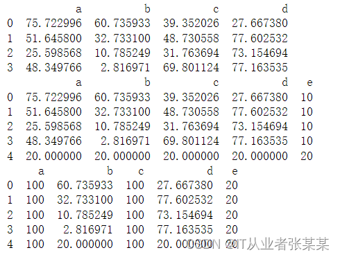
# 添加与修改 df = pd.DataFrame(np.random.rand(16).reshape(4,4)*100, columns = ['a','b','c','d']) print(df) df['e'] = 10 df.loc[4] = 20 print(df) # 新增列/行并赋值 df['e'] = 20 df[['a','c']] = 100 print(df) # 索引后直接修改值- 1
- 2
- 3
- 4
- 5
- 6
- 7
- 8
- 9
- 10
- 11
- 12
- 13
- 14
输出为:
 删除:
删除:# 删除 del / drop() df = pd.DataFrame(np.random.rand(16).reshape(4,4)*100, columns = ['a','b','c','d']) print(df) del df['a'] print(df) print('-----') # del语句 - 删除列 print(df.drop(0)) print(df.drop([1,2])) print(df) print('-----') # drop()删除行,inplace=False → 删除后生成新的数据,不改变原数据 print(df.drop(['d'], axis = 1)) print(df) # drop()删除列,需要加上axis = 1,inplace=False → 删除后生成新的数据,不改变原数据- 1
- 2
- 3
- 4
- 5
- 6
- 7
- 8
- 9
- 10
- 11
- 12
- 13
- 14
- 15
- 16
- 17
- 18
- 19
- 20
输出为:
- 对齐
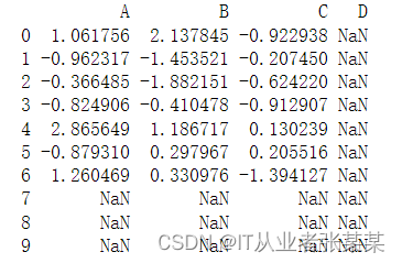
# 对齐 df1 = pd.DataFrame(np.random.randn(10, 4), columns=['A', 'B', 'C', 'D']) df2 = pd.DataFrame(np.random.randn(7, 3), columns=['A', 'B', 'C']) print(df1 + df2) # DataFrame对象之间的数据自动按照列和索引(行标签)对齐- 1
- 2
- 3
- 4
- 5
- 6
输出为:
- /排序
- 排序1 - 按值排序 .sort_values
pandas中可以使用sort_values()方法将Series、DataFrmae类对象按值的大小排序。
DataFrame.sort_values(by, axis=0, ascending=True, inplace=False, kind='quicksort', na_position='last', ignore_index=False)- 1
- 2
by:表示根据指定的列索引名(axis=0或’index’)或行索引名(axis=1或’columns’)进行排序。
axis:表示轴编号(排序的方向),0代表按行排序,1代表按列排序。
ascending:表示是否以升序方式排序,默认为True。若设置为False,则表示按降序方式排序。
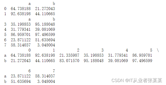
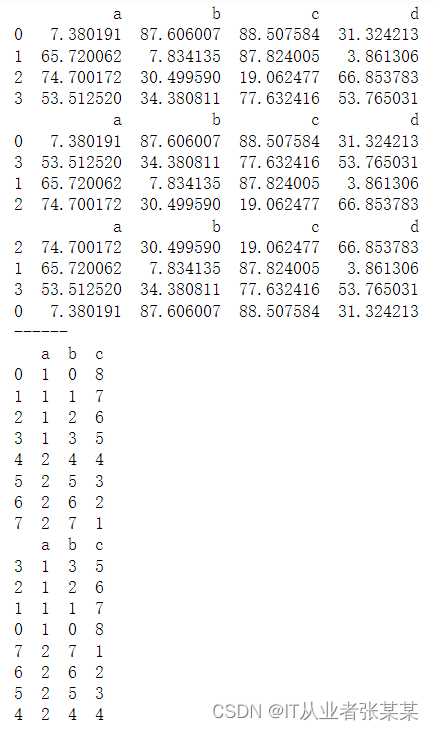
na_position:表示缺失值的显示位置,可以取值为’first’(首位)或’last’(末位)。# 排序1 - 按值排序 .sort_values # 同样适用于Series df1 = pd.DataFrame(np.random.rand(16).reshape(4,4)*100, columns = ['a','b','c','d']) print(df1) print(df1.sort_values(['a'], ascending = True)) # 升序 print(df1.sort_values(['a'], ascending = False)) # 降序 print('------') # ascending参数:设置升序降序,默认升序 # 单列排序 df2 = pd.DataFrame({'a':[1,1,1,1,2,2,2,2], 'b':list(range(8)), 'c':list(range(8,0,-1))}) print(df2) print(df2.sort_values(['a','c'])) # 多列排序,按列顺序排序- 1
- 2
- 3
- 4
- 5
- 6
- 7
- 8
- 9
- 10
- 11
- 12
- 13
- 14
- 15
- 16
- 17
- 18
输出为:
- 排序2 - 索引排序 .sort_index
pandas中提供了一个sort_index()方法,使用sort_index()方法可以让Series类对象DataFrame类对象按索引的大小进行排序。
sort_index(axis=0, level=None, ascending=True, inplace=False, kind='quicksort', na_position='last', sort_remaining=True, ignore_index: bool = False)- 1
- 2
- 3
axis:表示轴编号(排序的方向),0代表按行排序,1代表按列排序。
level:表示按哪个索引层级排序,默认为None。
ascending:表示是否以升序方式排序,默认为True。若设置为False,则表示按降序方式排序。
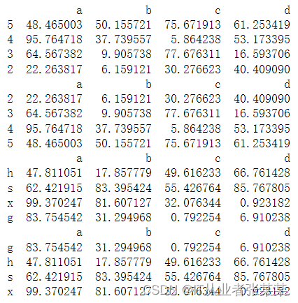
kind:表示排序算法,可以取值为’quicksort’、 'mergesort’或’heapsort’,默认为‘quicksort’。# 排序2 - 索引排序 .sort_index df1 = pd.DataFrame(np.random.rand(16).reshape(4,4)*100, index = [5,4,3,2], columns = ['a','b','c','d']) df2 = pd.DataFrame(np.random.rand(16).reshape(4,4)*100, index = ['h','s','x','g'], columns = ['a','b','c','d']) print(df1) print(df1.sort_index()) print(df2) print(df2.sort_index()) # 按照index排序 # 默认 ascending=True, inplace=False- 1
- 2
- 3
- 4
- 5
- 6
- 7
- 8
- 9
- 10
- 11
- 12
- 13
- 14
输出为:
1.5 Index索引对象
1.5.1 索引对象概述
Index类的常见子类,包括MultiIndex、Int64Index、DatetimeIndex等
掌握分层索引,可以通过多种方式熟练地创建分层索引。
在创建Series类对象或DataFrame类对象时,既可以使用自动生成的整数索引,也可以使用自定义的标签索引。无论哪种形式的索引,都是一个Index类的对象。
Index是一个基类,它派生了许多子类。
 Int64Index、Float64Index、DatetimeIndex和PeriodIndex只能被用于创建单层索引(轴方向上只有一层结构的索引),MultiIndex类代表分层索引,即轴方向上有两层或两层以上结构的索引。
 创建分层索引方法如下:

1.5.2 索引对象操作
- 设置索引
In [8]: info = pd.DataFrame([('William', 'C'), ('Smith', 'Java'), ('Parker', 'Python'), ('Phill', np.nan)], index=[1, 2, 3, 4], columns=('name', 'Language')) info- 1
- 2
- 3
输出为:
Out[8]: name Language 1 William C 2 Smith Java 3 Parker Python 4 Phill NaN- 1
- 2
- 3
- 4
- 5
- 6
- 设置索引
set_index() 将已存在的列标签设置为 DataFrame 行索引。除了可以添加索引外,也可以替换已经存在的索引。比如您也可以把 Series 或者一个 DataFrme 设置成另一个 DataFrame 的索引。示例如下:
In [6]: import pandas as pd import numpy as np info = pd.DataFrame({'Name': ['Parker', 'Terry', 'Smith', 'William'], 'Year': [2011, 2009, 2014, 2010], 'Leaves': [10, 15, 9, 4]}) info.set_index('Name')- 1
- 2
- 3
- 4
- 5
输出为:
Out[6]: Year Leaves Name Parker 2011 10 Terry 2009 15 Smith 2014 9 William 2010 4- 1
- 2
- 3
- 4
- 5
- 6
- 7
- 重置索引
您可以使用 reset_index() 来恢复初始行索引,示例如下:
In [11]: info = pd.DataFrame([('William', 'C'), ('Smith', 'Java'), ('Parker', 'Python'), ('Phill', np.nan)], index=[1, 2, 3, 4], columns=('name', 'Language')) info- 1
- 2
- 3
输出为:
Out[11]: name Language 1 William C 2 Smith Java 3 Parker Python 4 Phill NaN- 1
- 2
- 3
- 4
- 5
- 6
In [13]: info.reset_index()- 1
输出为:
Out[13]: index name Language 0 1 William C 1 2 Smith Java 2 3 Parker Python 3 4 Phill NaN- 1
- 2
- 3
- 4
- 5
- 6
- 重新索引
重新索引是重新为原对象设定索引,以构建一个符合新索引的对象。pandas中使用reindex()方法实现重新索引功能,该方法会参照原有的Series类对象或DataFrame类对象的索引设置数据:若该索引存在于新对象中,则其对应的数据设为原数据,否则填充为缺失值NaN。
reindex(labels=None, index=None, columns=None, axis=None, method=None, copy=True, level=None, fill_value=nan, limit=None, tolerance=None)- 1
- 2
- 3
index:表示新的行索引。
colums:表示新的列索引。
method:表示缺失值的填充方式,支持’None’(默认值)、‘fill或pad’、‘bfill或backfill’、'nearest’这几个值,其中’None’代表不填充缺失值;fill或pad’代表前向填充缺失值;'bfill或backfill’代表后向填充缺失值;'nearest’代表根据最近的值填充缺失值。
fill_vlaue:表示缺失值的替代值。
limit:表示前向或者后向填充的最大填充量。In [18]: index = ['Firefox', 'Chrome', 'Safari', 'IE10', 'Konqueror'] df = pd.DataFrame({'http_status': [200, 200, 404, 404, 301],'response_time': [0.04, 0.02, 0.07, 0.08, 1.0]},index=index) df- 1
- 2
- 3
- 4
输出为:
Out[18]: http_status response_time Firefox 200 0.04 Chrome 200 0.02 Safari 404 0.07 IE10 404 0.08 Konqueror 301 1.00- 1
- 2
- 3
- 4
- 5
- 6
- 7
In [21: new_index = ['Safari', 'Iceweasel', 'Comodo Dragon', 'IE10','Chrome'] new_df = df.reindex(new_index) new_df- 1
- 2
- 3
- 4
输出为:
Out[21]: http_status response_time Safari 404.0 0.07 Iceweasel NaN NaN Comodo Dragon NaN NaN IE10 404.0 0.08 Chrome 200.0 0.02- 1
- 2
- 3
- 4
- 5
- 6
- 7
In [22]: new_df = df.reindex(new_index, fill_value='missing') new_df # 通过fill_value参数,使用指定值对缺失值进行填充- 1
- 2
- 3
输出为:
Out[23]: http_status response_time Safari 404 0.07 Iceweasel missing missing Comodo Dragon missing missing IE10 404 0.08 Chrome 200 0.02- 1
- 2
- 3
- 4
- 5
- 6
- 7
In [25]: col_df = df.reindex(columns=['http_status', 'user_agent']) col_df- 1
- 2
- 3
输出为
Out[25]: http_status user_agent Firefox 200 NaN Chrome 200 NaN Safari 404 NaN IE10 404 NaN Konqueror 301 NaN- 1
- 2
- 3
- 4
- 5
- 6
- 7
1.5.3 使用索引对象操作数据
1.5.3.1 使用单层索引访问数据
无论是创建Series类对象还是创建DataFrame类对象,根本目的在于对Series类对象或DataFrame类对象中的数据进行处理,但在处理数据之前,需要先访问Series类对象或DataFrame类对象中的数据。
pandas中可以使用[]、loc、iloc、at和iat这几种方式访问Series类对象和DataFrame类对象的数据。- 使用[]访问数据
变量[索引]- 1
需要说明的是,若变量的值是一个Series类对象,则会根据索引获取该对象中对应的单个数据;若变量的值是一个DataFrame类对象,在使用“[索引]”访问数据时会将索引视为列索引,进而获取该列索引对应的一列数据。
- 使用loc和iloc访问数据
pandas中也可以使用loc和iloc访问数据。
变量.loc[索引] 变量.iloc[索引]- 1
- 2
以上方式中,"loc[索引]"中的索引必须为自定义的标签索引,而"iloc[索引]"中的索引必须为自动生成的整数索引。需要说明的是,若变量是一个DataFrame类对象,它在使用"loc[索引]"或"iloc[索引]"访问数据时会将索引视为行索引,获取该索引对应的一行数据。
- 使用at和iat访问数据
pandas中还可以使用at和iat访问数据,与前两种方式相比,这种方式可以访问DataFrame类对象的单个数据。
变量.at[行索引, 列索引] 变量.iat[行索引, 列索引]- 1
- 2
以上方式中,"at[行索引, 列索引]"中的索引必须为自定义的标签索引,"iat[行索引, 列索引]"中的索引必须为自动生成的整数索引。
1.5.3.2 使用分层索引访问数据
掌握分层索引的使用方式,可以通过[]、loc和iloc访问Series类对象和DataFrame类对象的数据
pandas中除了可以通过简单的单层索引访问数据外,还可以通过复杂的分层索引访问数据。与单层索引相比,分层索引只适用于[]、loc和iloc,且用法大致相同。- 使用[]访问数据
由于分层索引的索引层数比单层索引多,在使用[]方式访问数据时,需要根据不同的需求传入不同层级的索引。
变量[第一层索引] 变量[第一层索引][第二层索引]- 1
- 2
以上方式中,使用
变量[第一层索引]- 1
可以访问第一层索引嵌套的第二层索引及其对应的数据;
使用变量[第一层索引][第二层索引]- 1
可以访问第二层索引对应的数据。
- 使用loc和iloc访问数据
使用iloc和loc也可以访问具有分层索引的Series类对象或DataFrame类对象。
变量.loc[第一层索引] # 访问第一层索引对应的数据 变量.loc[第一层索引][第二层索引] # 访问第二层索引对应的数据 变量.iloc[整数索引] # 访问第二层索引对应的数据- 1
- 2
- 3
1.6 统计计算与统计描述
1.6.1 常见的统计计算函数

import pandas as pd import numpy as np df = pd.DataFrame({'col_A':[2,34,25,4], 'col_B':[0,3,45,9], 'col_C':[7,5,5,3]}, index=['A','B','C','D']) df- 1
- 2
- 3
- 4
- 5
- 6
- 7
输出为:
col_A col_B col_C A 2 0 7 B 34 3 5 C 25 45 5 D 4 9 3- 1
- 2
- 3
- 4
- 5
df.idxmax() # 获取每列最大值对应的行索引- 1
输出为:
col_A B col_B C col_C A dtype: object- 1
- 2
- 3
- 4
1.6.2 统计描述
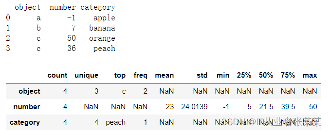
如果希望一次性描述Series类对象或DataFrame类对象的多个统计指标,如平均值、最大值、最小值等,那么可以使用describe()方法实现,而不用逐个调用统计计算函数。
describe(percentiles=None, include=None, exclude=None)- 1
percentiles:表示结果包含的百分数,位于[0,1]之间。若不设置该参数,则默认为[0.25,0.5,0.75],即展示25%、50%、75%分位数。
include:表示结果中包含数据类型的白名单,默认为None。
exclude:表示结果中忽略数据类型的黑名单,默认为None。df_obj = pd.DataFrame({'object':['a', 'b', 'c', 'c'], 'number':[-1, 7, 50, 36], 'category':pd.Categorical(['apple', 'banana', 'orange', 'peach'])}) print(df_obj) # df_obj.describe().T # df_obj.describe(include=['O']).T df_obj.describe(include='all').T- 1
- 2
- 3
- 4
- 5
- 6
- 7
输出为:
1.7 绘制图形
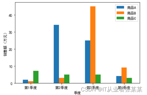
pandas的DataFrame类对象和Series类对象中提供了一个plot()方法,使用该方法可以快速地绘制一些常见的图表,包括折线图、柱形图、条形图、直方图、箱形图、饼图等。
plot(x=None, y=None, kind='line', ax=None, subplots=False, sharex=None, sharey=False, layout=None,figsize=None, use_index=True, title=None, grid=None, legend=True, style=None, logx=False, logy=False, loglog=False, xlabel=None, ylabel=None, xlim=None, ylim=None, rot=None,xerr=None,secondary_y=False, sort_columns=False, **kwargs)- 1
- 2
- 3
- 4
kind:表示绘图的类型。
figsize:表示图表尺寸的大小,接收形式如(宽度,高度)的元组。
title:表示图表的标题。
xlabel:表示x轴的标签。
ylabel:表示y轴的标签。
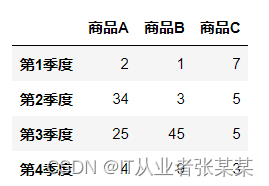
rot:表示轴标签旋转的角度。import pandas as pd df = pd.DataFrame({'商品A':[2,34,25,4], '商品B':[1,3,45,9], '商品C':[7,5,5,3]}, index=['第1季度','第2季度','第3季度','第4季度']) df- 1
- 2
- 3
- 4
- 5
- 6
输出为:
# 导入matplotlib库 import matplotlib.pyplot as plt # 设置显示中文 plt.rcParams['font.sans-serif'] = ['SimHei'] df.plot(kind='bar', xlabel='季度', ylabel='销售额(万元)', rot=0) plt.show()- 1
- 2
- 3
- 4
- 5
- 6
输出为:
-
相关阅读:
时钟有关概念汇总
TCP/IP 原理、实现方式与优缺点
使用MONAI轻松加载医学公开数据集,包括医学分割十项全能挑战数据集和MedMNIST分类数据集
SMP多核启动(一):spin-table
软件测试基础理论知识—用例篇
Codeforces Round 900 (Div. 3)
浅谈斜率优化
子查询作为检索表时的不同使用场景以及是否需要添加别名的问题
Q-REG论文阅读
Android---屏幕适配的处理技巧
- 原文地址:https://blog.csdn.net/m0_38139250/article/details/126747621
