-
机器学习实训(3)——训练模型(补充)
目录
本篇博文是对训练模型的补充:
机器学习实战(4)——训练模型_WHJ226的博客-CSDN博客
1 基础知识
- 如果我们的训练集有超过百万个特征,我们该选择什么线性回归训练算法?
我们可以使用随机梯度下降和小批量梯度下降,由于计算复杂度随着特征数量的增加而快速提升,因此不能使用标准方程。
- 如果我们的训练集里特征的数值大小迥异,什么算法可能会受到影响?
梯度下降算法,进行特征缩放即可。
- 训练逻辑回归模型时,梯度下降是否会困于局部最小值?
不会,因为成本函数是凸函数。
- 假设运行时间足够长,所有梯度下降算法是不是最终产生相同的模型?
如果优化问题是凸的,并且学习率也不是太高,那么所有梯度下降算法都可以接近全局最优,最终生成的模型都非常相似。但是除非降低学习率,否则随机梯度下降和小批量梯度下降都不会真正收敛,相反,它们会不断在全局最优的附近波动。
- 如果你使用的是批量梯度下降,并且每一轮训练都绘制出其验证误差,如果发现验证误差持续上升,可能会发生什么?
如果验证误差开始上升,可能之一是学习率太高,算法开始发散导致;如果训练误差开始上升,显然需要我们降低学习率。但是,如果训练误差没有上升,那么模型可能过度拟合训练集。
- 当验证误差开始上升时,立刻停止小批量梯度下降算法训练是否可行?
由于随机性,它们不能保证在每一次的训练迭代中都取得进展,所以可能会过早停止训练。我们可以定时保存模型,当较长一段时间都没有改善时,可以恢复到保存的最优模型。
- 哪种梯度下降算法能最快达到最优解的附近?哪种会收敛?
随机梯度下降的训练迭代最快,但是只有批量梯度下降才会经过足够长的时间训练后真正收敛。对于随机梯度下降和小批量梯度下降,我们需要降低学习率使其收敛。
- 假设我们使用的是多项式回归,绘制出学习曲线,发现训练误差和验证误差之间存在很大的差距,是发生了什么,如何解决?
如果验证误差高于训练误差,可能是因为模型过度拟合训练集。我们可以对多项式降阶:自由度越低的模型,过度拟合的可能性越低,或者施加正则化,在成本函数中增加岭回归或LASSO回归。
- 假设我们使用的是岭回归,训练误差和验证误差几乎相等,并且非常高。模型是高方差还是高偏差?
可能模型对训练集拟合不足,偏差较高,可以尝试降低正则化超参数。
- 如下:
为何使用岭回归而不是线性回归?
有正则化的模型通常比没有正则化的模型表现得好。
Lasso回归而不是岭回归?
Lasso回归倾向于将不重要特征权重将至0。这是执行特征选择的一种方法。
弹性网络而不是 Lasso回归?
某些情况下,Lasso回归可能产生异常表现(例如多个特征强相关或特征数量比训练实例多),并且,弹性网络会添加一个超参数来对模型进行调整。
2 Softmax回归中实现早期停止的批量梯度下降
我们将以鸢尾花数据集为例:
首先,加载数据:
- from sklearn import datasets
- iris = datasets.load_iris()
- X = iris["data"][:, (2, 3)] # 花瓣长度和宽度特征
- y = iris["target"]
为每个实例添加偏置项:
- import numpy as np
- X_with_bias = np.c_[np.ones([len(X), 1]), X]
有关numpy和np.ones()的用法参考该博文:机器学习(1)——Python数据处理与绘图_WHJ226的博客-CSDN博客_python数据画图
设置随机种子,实现结果复现:
np.random.seed(42)我们通常是使用 Scikit-Learn的train_test_split()函数来划分数据集的,现在我们不使用该函数来实现数据集的划分,让我们看一下:
- #设置比例
- test_ratio = 0.2
- validation_ratio = 0.2
- total_size = len(X_with_bias)
- #数量
- test_size = int(total_size * test_ratio)
- validation_size = int(total_size * validation_ratio)
- train_size = total_size - test_size - validation_size
- #数据洗牌,
- rnd_indices = np.random.permutation(total_size) #生成一组重新排列的数组
- #数据集划分
- X_train = X_with_bias[rnd_indices[:train_size]]
- y_train = y[rnd_indices[:train_size]]
- X_valid = X_with_bias[rnd_indices[train_size:-test_size]]
- y_valid = y[rnd_indices[train_size:-test_size]]
- X_test = X_with_bias[rnd_indices[-test_size:]]
- y_test = y[rnd_indices[-test_size:]]
目标是目前的类指数(0,1或2),但我们需要目标类概率来训练Softmax回归模型。每个实例的目标类概率将等于0.0,除了目标类的概率为1.0。让我们写一个函数来将类索引的向量转换为一个包含每个实例的一个 one-hot 矩阵,并在前10个实例上测试这个函数:
- def to_one_hot(y):
- n_classes = y.max() + 1
- m = len(y)
- Y_one_hot = np.zeros((m, n_classes))
- Y_one_hot[np.arange(m), y] = 1
- return Y_one_hot
- #查看
- y_train[:10]
运行结果如下:
array([0, 1, 2, 1, 1, 0, 1, 1, 1, 0])尝试转换:
to_one_hot(y_train[:10])运行结果如下:
- array([[0., 1., 0.],
- [1., 0., 0.],
- [0., 0., 1.],
- [0., 1., 0.],
- [0., 1., 0.],
- [1., 0., 0.],
- [0., 1., 0.],
- [0., 0., 1.],
- [0., 1., 0.],
- [0., 1., 0.]])
下面,让我们为训练集和测试集创建目标类概率矩阵:
- Y_train_one_hot = to_one_hot(y_train)
- Y_valid_one_hot = to_one_hot(y_valid)
- Y_test_one_hot = to_one_hot(y_test)
现在让我们实现Softmax功能。回想一下,它是由以下方程定义的:

- def softmax(logits):
- exps = np.exp(logits)
- exp_sums = np.sum(exps, axis=1, keepdims=True)
- return exps / exp_sums
然后,我们需要定义输入和输出的数量:
- n_inputs = X_train.shape[1] # == 3 (2 features plus the bias term)
- n_outputs = len(np.unique(y_train)) # == 3 (3 iris classes)
以下就开始训练部分了,首先是成本函数:

通过最小化成本函数实现对目标类别做出高概率的模型。
以下是梯度向量:
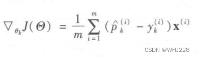
注意,如果p^(i)k=0, log(p^(i)k)可能无法计算。因此,我们将对log(p^(i)k)增加一个极小的值,以避免得到nan值。
下面是代码实现:
- eta = 0.01
- n_iterations = 5001
- m = len(X_train)
- epsilon = 1e-7
- Theta = np.random.randn(n_inputs, n_outputs)
- for iteration in range(n_iterations):
- logits = X_train.dot(Theta)
- Y_proba = softmax(logits)
- loss = -np.mean(np.sum(Y_train_one_hot * np.log(Y_proba + epsilon), axis=1))
- error = Y_proba - Y_train_one_hot
- if iteration % 500 == 0:
- print(iteration, loss)
- gradients = 1/m * X_train.T.dot(error)
- Theta = Theta - eta * gradients
运行结果如下:
- 0 3.5356045081790177
- 500 0.7698276617097016
- 1000 0.6394784332731978
- 1500 0.5618741363839648
- 2000 0.5095831080853224
- 2500 0.471273775599093
- 3000 0.44155863305230325
- 3500 0.4175598664804123
- 4000 0.3975941721521857
- 4500 0.38060484552797946
- 5000 0.3658905593000994
让我们看看模型参数:
Theta运行结果如下:
- array([[ 2.44942005, -1.63172695, -3.63642175],
- [-0.61947541, 0.50273412, 0.22142236],
- [-0.96378971, 0.39312153, 2.48742003]])
现在让我们对验证集进行预测,并检查准确性得分:
- logits = X_valid.dot(Theta)
- Y_proba = softmax(logits)
- y_predict = np.argmax(Y_proba, axis=1)
- accuracy_score = np.mean(y_predict == y_valid)
- accuracy_score
运行结果如下:
0.9333333333333333这个模型看起来不错。为了练习的目的,让我们添加一些ℓ2的正则化。下面的训练代码与上面的代码类似,但损失现在有一个额外的ℓ2惩罚,梯度有适当的额外项(注意,我们没有正则化Theta的第一个元素,因为它对应于偏差项)。同时,让我们尝试提高学习率eta。
- eta = 0.1
- n_iterations = 5001
- m = len(X_train)
- epsilon = 1e-7
- alpha = 0.1 # regularization hyperparameter
- Theta = np.random.randn(n_inputs, n_outputs)
- for iteration in range(n_iterations):
- logits = X_train.dot(Theta)
- Y_proba = softmax(logits)
- xentropy_loss = -np.mean(np.sum(Y_train_one_hot * np.log(Y_proba + epsilon), axis=1))
- l2_loss = 1/2 * np.sum(np.square(Theta[1:]))
- loss = xentropy_loss + alpha * l2_loss
- error = Y_proba - Y_train_one_hot
- if iteration % 500 == 0:
- print(iteration, loss)
- gradients = 1/m * X_train.T.dot(error) + np.r_[np.zeros([1, n_outputs]), alpha * Theta[1:]]
- Theta = Theta - eta * gradients
运行结果如下:
- 0 4.074160805836161
- 500 0.5159746132958637
- 1000 0.49124622842160703
- 1500 0.4842826626269516
- 2000 0.48172881149189384
- 2500 0.4807092367289707
- 3000 0.4802846688736693
- 3500 0.48010354679755285
- 4000 0.4800251331504283
- 4500 0.4799908689215818
- 5000 0.4799758070182931
由于额外的ℓ2惩罚,损失似乎比之前更大,但也许这个模型会表现得更好?让我们来看看:
- logits = X_valid.dot(Theta)
- Y_proba = softmax(logits)
- y_predict = np.argmax(Y_proba, axis=1)
- accuracy_score = np.mean(y_predict == y_valid)
- accuracy_score
运行结果如下:
0.9333333333333333我们恰巧选用的验证集可能不太完美,不过没关系。
现在让我们加入早起停止。为此,我们只需要在每次迭代中测量验证集上的损失,并在错误开始增长时停止。
- eta = 0.1
- n_iterations = 5001
- m = len(X_train)
- epsilon = 1e-7
- alpha = 0.1 # regularization hyperparameter
- best_loss = np.infty
- Theta = np.random.randn(n_inputs, n_outputs)
- for iteration in range(n_iterations):
- logits = X_train.dot(Theta)
- Y_proba = softmax(logits)
- xentropy_loss = -np.mean(np.sum(Y_train_one_hot * np.log(Y_proba + epsilon), axis=1))
- l2_loss = 1/2 * np.sum(np.square(Theta[1:]))
- loss = xentropy_loss + alpha * l2_loss
- error = Y_proba - Y_train_one_hot
- gradients = 1/m * X_train.T.dot(error) + np.r_[np.zeros([1, n_outputs]), alpha * Theta[1:]]
- Theta = Theta - eta * gradients
- logits = X_valid.dot(Theta)
- Y_proba = softmax(logits)
- xentropy_loss = -np.mean(np.sum(Y_valid_one_hot * np.log(Y_proba + epsilon), axis=1))
- l2_loss = 1/2 * np.sum(np.square(Theta[1:]))
- loss = xentropy_loss + alpha * l2_loss
- if iteration % 500 == 0:
- print(iteration, loss)
- if loss < best_loss:
- best_loss = loss
- else:
- print(iteration - 1, best_loss)
- print(iteration, loss, "early stopping!")
- break
运行结果如下:
- 0 1.7715206020472196
- 500 0.5707532983595428
- 1000 0.545946882198638
- 1500 0.5380948912189549
- 2000 0.5349265834600064
- 2500 0.5335454107098025
- 3000 0.5329073608729564
- 3500 0.5325963465739497
- 4000 0.5324366553661258
- 4500 0.5323504675033873
- 5000 0.5323017576862805
我们再来看看这个模型:
- logits = X_valid.dot(Theta)
- Y_proba = softmax(logits)
- y_predict = np.argmax(Y_proba, axis=1)
- accuracy_score = np.mean(y_predict == y_valid)
- accuracy_score
运行结果如下:
0.9333333333333333现在让我们在整个数据集上绘制模型的预测:
- # To plot pretty figures
- %matplotlib inline
- import matplotlib as mpl
- import matplotlib.pyplot as plt
- mpl.rc('axes', labelsize=14)
- mpl.rc('xtick', labelsize=12)
- mpl.rc('ytick', labelsize=12)
- x0, x1 = np.meshgrid(
- np.linspace(0, 8, 500).reshape(-1, 1),
- np.linspace(0, 3.5, 200).reshape(-1, 1),
- )
- X_new = np.c_[x0.ravel(), x1.ravel()]
- X_new_with_bias = np.c_[np.ones([len(X_new), 1]), X_new]
- logits = X_new_with_bias.dot(Theta)
- Y_proba = softmax(logits)
- y_predict = np.argmax(Y_proba, axis=1)
- zz1 = Y_proba[:, 1].reshape(x0.shape)
- zz = y_predict.reshape(x0.shape)
- plt.figure(figsize=(10, 4))
- plt.plot(X[y==2, 0], X[y==2, 1], "g^", label="Iris-Virginica")
- plt.plot(X[y==1, 0], X[y==1, 1], "bs", label="Iris-Versicolor")
- plt.plot(X[y==0, 0], X[y==0, 1], "yo", label="Iris-Setosa")
- from matplotlib.colors import ListedColormap
- custom_cmap = ListedColormap(['#fafab0','#9898ff','#a0faa0'])
- plt.contourf(x0, x1, zz, cmap=custom_cmap)
- contour = plt.contour(x0, x1, zz1, cmap=plt.cm.brg)
- plt.clabel(contour, inline=1, fontsize=12)
- plt.xlabel("Petal length", fontsize=14)
- plt.ylabel("Petal width", fontsize=14)
- plt.legend(loc="upper left", fontsize=14)
- plt.axis([0, 7, 0, 3.5])
- plt.show()
运行结果如下:

现在我们来看看最终模型在测试集上的准确性:
- logits = X_test.dot(Theta)
- Y_proba = softmax(logits)
- y_predict = np.argmax(Y_proba, axis=1)
- accuracy_score = np.mean(y_predict == y_test)
- accuracy_score
运行结果如下:
0.9666666666666667不错,不过模型有一点不完美。这种可变性可能是由于数据集非常小:根据我们如何对训练集、验证集和测试集进行抽样,可以得到截然不同的结果。如果尝试更改随机种子并再次运行代码几次,我们将看到结果会有所不同。
学习笔记——《机器学习实战:基于Scikit-Learn和TensorFlow》
-
相关阅读:
我梦想中的学习组织-勤学会
matlab绘制雷达图
mac 容器化 安装docker & es | redis
Kylin v10安装DM8数据库
Apache Shiro 集成-spring
IDEA自定义代码快捷指令
C语言-入门-extern和头文件(十六)
电脑重装系统后鼠标动不了该怎么解决
【MySQL·水滴计划】第三话- SQL的基本概念
Could not find artifact com.sleepycat;je:jar:7.3.7 in aliyunmaven
- 原文地址:https://blog.csdn.net/WHJ226/article/details/126708480
