-
【OpenCV】Chapter7.图像噪声与滤波器
最近想对OpenCV进行系统学习,看到网上这份教程写得不错,于是跟着来学习实践一下。
【youcans@qq.com, youcans 的 OpenCV 例程, https://youcans.blog.csdn.net/article/details/125112487】
程序仓库:https://github.com/zstar1003/OpenCV-Learning添加噪声
高斯噪声
高斯噪声的概率密度函数为:

示例程序:""" 高斯噪声 """ import cv2 import matplotlib.pyplot as plt import numpy as np img = cv2.imread("../img/lena.jpg", 1) mu, sigma = 0.0, 20.0 noiseGause = np.random.normal(mu, sigma, img.shape) imgGaussNoise = img + noiseGause imgGaussNoise = np.uint8(cv2.normalize(imgGaussNoise, None, 0, 255, cv2.NORM_MINMAX)) # 归一化为 [0,255] plt.figure(figsize=(9, 3)) plt.subplot(131), plt.title("Origin"), plt.axis('off') plt.imshow(img, 'gray', vmin=0, vmax=255) plt.subplot(132), plt.title("GaussNoise"), plt.axis('off') plt.imshow(imgGaussNoise, 'gray') plt.subplot(133), plt.title("Gray Hist") histNP, bins = np.histogram(imgGaussNoise.flatten(), bins=255, range=[0, 255], density=True) plt.bar(bins[:-1], histNP[:]) plt.tight_layout() plt.show()- 1
- 2
- 3
- 4
- 5
- 6
- 7
- 8
- 9
- 10
- 11
- 12
- 13
- 14
- 15
- 16
- 17
- 18
- 19
- 20
- 21
- 22
- 23
- 24
- 25

瑞利噪声
瑞利噪声的概率密度函数为

示例程序:""" 瑞利噪声 """ import cv2 import matplotlib.pyplot as plt import numpy as np img = cv2.imread("../img/lena.jpg", 0) a = 30.0 noiseRayleigh = np.random.rayleigh(a, size=img.shape) imgRayleighNoise = img + noiseRayleigh imgRayleighNoise = np.uint8(cv2.normalize(imgRayleighNoise, None, 0, 255, cv2.NORM_MINMAX)) # 归一化为 [0,255] plt.figure(figsize=(9, 3)) plt.subplot(131), plt.title("Origin"), plt.axis('off') plt.imshow(img, 'gray', vmin=0, vmax=255) plt.subplot(132), plt.title("RayleighNoise"), plt.axis('off') plt.imshow(imgRayleighNoise, 'gray') plt.subplot(133), plt.title("Gray Hist") histNP, bins = np.histogram(imgRayleighNoise.flatten(), bins=255, range=[0, 255], density=True) plt.bar(bins[:-1], histNP[:]) plt.tight_layout() plt.show()- 1
- 2
- 3
- 4
- 5
- 6
- 7
- 8
- 9
- 10
- 11
- 12
- 13
- 14
- 15
- 16
- 17
- 18
- 19
- 20
- 21
- 22
- 23
- 24
- 25

伽马噪声
伽马噪声又称爱尔兰噪声,其概率密度函数为

示例程序:""" 伽马噪声 """ import cv2 import matplotlib.pyplot as plt import numpy as np img = cv2.imread("../img/lena.jpg", 0) a, b = 10.0, 2.5 noiseGamma = np.random.gamma(shape=b, scale=a, size=img.shape) imgGammaNoise = img + noiseGamma imgGammaNoise = np.uint8(cv2.normalize(imgGammaNoise, None, 0, 255, cv2.NORM_MINMAX)) # 归一化为 [0,255] plt.figure(figsize=(9, 3)) plt.subplot(131), plt.title("Origin"), plt.axis('off') plt.imshow(img, 'gray', vmin=0, vmax=255) plt.subplot(132), plt.title("Gamma noise"), plt.axis('off') plt.imshow(imgGammaNoise, 'gray') plt.subplot(133), plt.title("Gray hist") histNP, bins = np.histogram(imgGammaNoise.flatten(), bins=255, range=[0, 255], density=True) plt.bar(bins[:-1], histNP[:]) plt.tight_layout() plt.show()- 1
- 2
- 3
- 4
- 5
- 6
- 7
- 8
- 9
- 10
- 11
- 12
- 13
- 14
- 15
- 16
- 17
- 18
- 19
- 20
- 21
- 22
- 23
- 24
- 25

指数噪声
指数噪声的概率密度函数为

示例程序:""" 指数噪声 """ import cv2 import matplotlib.pyplot as plt import numpy as np img = cv2.imread("../img/lena.jpg", 0) a = 10.0 noiseExponent = np.random.exponential(scale=a, size=img.shape) imgExponentNoise = img + noiseExponent imgExponentNoise = np.uint8(cv2.normalize(imgExponentNoise, None, 0, 255, cv2.NORM_MINMAX)) # 归一化为 [0,255] plt.figure(figsize=(9, 3)) plt.subplot(131), plt.title("Origin"), plt.axis('off') plt.imshow(img, 'gray', vmin=0, vmax=255) plt.subplot(132), plt.title("Exponential noise"), plt.axis('off') plt.imshow(imgExponentNoise, 'gray') plt.subplot(133), plt.title("Gray hist") histNP, bins = np.histogram(imgExponentNoise.flatten(), bins=255, range=[0, 255], density=True) plt.bar(bins[:-1], histNP[:]) plt.tight_layout() plt.show()- 1
- 2
- 3
- 4
- 5
- 6
- 7
- 8
- 9
- 10
- 11
- 12
- 13
- 14
- 15
- 16
- 17
- 18
- 19
- 20
- 21
- 22
- 23
- 24
- 25

均匀噪声
均匀噪声的概率密度函数为

示例程序:
""" 均匀噪声 """ import cv2 import matplotlib.pyplot as plt import numpy as np img = cv2.imread("../img/lena.jpg", 0) mean, sigma = 10, 100 a = 2 * mean - np.sqrt(12 * sigma) # a = -14.64 b = 2 * mean + np.sqrt(12 * sigma) # b = 54.64 noiseUniform = np.random.uniform(a, b, img.shape) imgUniformNoise = img + noiseUniform imgUniformNoise = np.uint8(cv2.normalize(imgUniformNoise, None, 0, 255, cv2.NORM_MINMAX)) # 归一化为 [0,255] plt.figure(figsize=(9, 3)) plt.subplot(131), plt.title("Origin"), plt.axis('off') plt.imshow(img, 'gray', vmin=0, vmax=255) plt.subplot(132), plt.title("Uniform noise"), plt.axis('off') plt.imshow(imgUniformNoise, 'gray') plt.subplot(133), plt.title("Gray hist") histNP, bins = np.histogram(imgUniformNoise.flatten(), bins=255, range=[0, 255], density=True) plt.bar(bins[:-1], histNP[:]) plt.tight_layout() plt.show()- 1
- 2
- 3
- 4
- 5
- 6
- 7
- 8
- 9
- 10
- 11
- 12
- 13
- 14
- 15
- 16
- 17
- 18
- 19
- 20
- 21
- 22
- 23
- 24
- 25
- 26
- 27

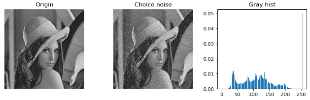
椒盐噪声
椒盐噪声的概率密度函数为

示例程序:
""" 椒盐噪声 """ import cv2 import matplotlib.pyplot as plt import numpy as np img = cv2.imread("../img/lena.jpg", 0) ps, pp = 0.05, 0.02 mask = np.random.choice((0, 0.5, 1), size=img.shape[:2], p=[pp, (1 - ps - pp), ps]) imgChoiceNoise = img.copy() imgChoiceNoise[mask == 1] = 255 imgChoiceNoise[mask == 0] = 0 plt.figure(figsize=(9, 3)) plt.subplot(131), plt.title("Origin"), plt.axis('off') plt.imshow(img, 'gray', vmin=0, vmax=255) plt.subplot(132), plt.title("Choice noise"), plt.axis('off') plt.imshow(imgChoiceNoise, 'gray') plt.subplot(133), plt.title("Gray hist") histNP, bins = np.histogram(imgChoiceNoise.flatten(), bins=255, range=[0, 255], density=True) plt.bar(bins[:-1], histNP[:]) plt.tight_layout() plt.show()- 1
- 2
- 3
- 4
- 5
- 6
- 7
- 8
- 9
- 10
- 11
- 12
- 13
- 14
- 15
- 16
- 17
- 18
- 19
- 20
- 21
- 22
- 23
- 24
- 25
- 26
滤波器
当图片中含有噪声时,可以采用滤波器来进行滤除。
算术平均滤波器
算术平均滤波器是最简单的均值滤波器,与空间域滤波中的盒式滤波器相同。
计算公式如下:

简单理解,就是将一个盒子中的每一个像素点以整个盒子的平均值替代。盒子尺寸越大就越模糊。
在OpenCV中可以用cv2.filter2D和cv2.boxFilter两种方式实现。示例程序:
""" 算术平均滤波器 """ import cv2 import matplotlib.pyplot as plt import numpy as np img = cv2.imread("../img/lena_noise.jpg", 0) kSize = (3, 3) kernalMean = np.ones(kSize, np.float32) / (kSize[0] * kSize[1]) # 生成归一化盒式核 imgConv1 = cv2.filter2D(img, -1, kernalMean) # cv2.filter2D 方法 kSize = (20, 20) imgConv3 = cv2.boxFilter(img, -1, kSize) # cv2.boxFilter 方法 (默认normalize=True) plt.figure(figsize=(9, 6)) plt.subplot(131), plt.axis('off'), plt.title("Original") plt.imshow(img, cmap='gray', vmin=0, vmax=255) plt.subplot(132), plt.axis('off'), plt.title("filter2D(kSize=[3,3])") plt.imshow(imgConv1, cmap='gray', vmin=0, vmax=255) plt.subplot(133), plt.axis('off'), plt.title("boxFilter(kSize=[20,20])") plt.imshow(imgConv3, cmap='gray', vmin=0, vmax=255) plt.tight_layout() plt.show()- 1
- 2
- 3
- 4
- 5
- 6
- 7
- 8
- 9
- 10
- 11
- 12
- 13
- 14
- 15
- 16
- 17
- 18
- 19
- 20
- 21
- 22
- 23
- 24
- 25

几何均值滤波器
几何均值滤波器计算公式如下:

这里和算术平均滤波器进行对比:
""" 几何均值滤波器 """ import cv2 import matplotlib.pyplot as plt import numpy as np img = cv2.imread("../img/lena_noise.jpg", 0) img_h = img.shape[0] img_w = img.shape[1] # 算术平均滤波 (Arithmentic mean filter) kSize = (3, 3) kernalMean = np.ones(kSize, np.float32) / (kSize[0] * kSize[1]) # 生成归一化盒式核 imgAriMean = cv2.filter2D(img, -1, kernalMean) # 几何均值滤波器 (Geometric mean filter) m, n = 3, 3 order = 1 / (m * n) kernalMean = np.ones((m, n), np.float32) # 生成盒式核 hPad = int((m - 1) / 2) wPad = int((n - 1) / 2) imgPad = np.pad(img.copy(), ((hPad, m - hPad - 1), (wPad, n - wPad - 1)), mode="edge") imgGeoMean = img.copy() for i in range(hPad, img_h + hPad): for j in range(wPad, img_w + wPad): prod = np.prod(imgPad[i - hPad:i + hPad + 1, j - wPad:j + wPad + 1] * 1.0) imgGeoMean[i - hPad][j - wPad] = np.power(prod, order) plt.figure(figsize=(9, 6)) plt.subplot(131), plt.axis('off'), plt.title("Original") plt.imshow(img, cmap='gray', vmin=0, vmax=255) plt.subplot(132), plt.axis('off'), plt.title("Arithmentic mean filter") plt.imshow(imgAriMean, cmap='gray', vmin=0, vmax=255) plt.subplot(133), plt.axis('off'), plt.title("Geometric mean filter") plt.imshow(imgGeoMean, cmap='gray', vmin=0, vmax=255) plt.tight_layout() plt.show()- 1
- 2
- 3
- 4
- 5
- 6
- 7
- 8
- 9
- 10
- 11
- 12
- 13
- 14
- 15
- 16
- 17
- 18
- 19
- 20
- 21
- 22
- 23
- 24
- 25
- 26
- 27
- 28
- 29
- 30
- 31
- 32
- 33
- 34
- 35
- 36
- 37
- 38
- 39
- 40
- 41
- 42

谐波平均滤波器
谐波平均滤波器计算公式如下:

谐波平均滤波器既能处理盐粒噪声(白色噪点),又能处理类似于高斯噪声的其他噪声,但不能处理胡椒噪声(黑色噪点)。""" 谐波平均滤波器 """ import cv2 import matplotlib.pyplot as plt import numpy as np img = cv2.imread("../img/lena_noise.jpg", 0) img_h = img.shape[0] img_w = img.shape[1] # 算术平均滤波 (Arithmentic mean filter) kSize = (3, 3) kernalMean = np.ones(kSize, np.float32) / (kSize[0] * kSize[1]) # 生成归一化盒式核 imgAriMean = cv2.filter2D(img, -1, kernalMean) # 谐波平均滤波器 (Harmonic mean filter) m, n = 3, 3 order = m * n kernalMean = np.ones((m, n), np.float32) # 生成盒式核 hPad = int((m - 1) / 2) wPad = int((n - 1) / 2) imgPad = np.pad(img.copy(), ((hPad, m - hPad - 1), (wPad, n - wPad - 1)), mode="edge") epsilon = 1e-8 imgHarMean = img.copy() for i in range(hPad, img_h + hPad): for j in range(wPad, img_w + wPad): sumTemp = np.sum(1.0 / (imgPad[i - hPad:i + hPad + 1, j - wPad:j + wPad + 1] + epsilon)) imgHarMean[i - hPad][j - wPad] = order / sumTemp plt.figure(figsize=(9, 6)) plt.subplot(131), plt.axis('off'), plt.title("Original") plt.imshow(img, cmap='gray', vmin=0, vmax=255) plt.subplot(132), plt.axis('off'), plt.title("Arithmentic mean filter") plt.imshow(imgAriMean, cmap='gray', vmin=0, vmax=255) plt.subplot(133), plt.axis('off'), plt.title("Harmonic mean filter") plt.imshow(imgHarMean, cmap='gray', vmin=0, vmax=255) plt.tight_layout() plt.show()- 1
- 2
- 3
- 4
- 5
- 6
- 7
- 8
- 9
- 10
- 11
- 12
- 13
- 14
- 15
- 16
- 17
- 18
- 19
- 20
- 21
- 22
- 23
- 24
- 25
- 26
- 27
- 28
- 29
- 30
- 31
- 32
- 33
- 34
- 35
- 36
- 37
- 38
- 39
- 40
- 41
- 42

反谐波平均滤波器
反谐波平均滤波器适用于降低或消除椒盐噪声,计算公式如下:
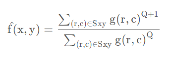
Q 称为滤波器的阶数,Q 取正整数时可以消除胡椒噪声,Q 取负整数时可以消除盐粒噪声,但不能同时消除这两种噪声。
反谐波平均滤波器当 Q=0 时简化为算术平均滤波器;当 Q=−1时简化为谐波平均滤波器。
示例程序:
""" 反谐波平均滤波器 """ import cv2 import matplotlib.pyplot as plt import numpy as np img = cv2.imread("../img/lena_noise.jpg", 0) img_h = img.shape[0] img_w = img.shape[1] m, n = 3, 3 order = m * n kernalMean = np.ones((m, n), np.float32) # 生成盒式核 hPad = int((m - 1) / 2) wPad = int((n - 1) / 2) imgPad = np.pad(img.copy(), ((hPad, m - hPad - 1), (wPad, n - wPad - 1)), mode="edge") Q = 1.5 # 反谐波平均滤波器 阶数 epsilon = 1e-8 imgHarMean = img.copy() imgInvHarMean = img.copy() for i in range(hPad, img_h + hPad): for j in range(wPad, img_w + wPad): # 谐波平均滤波器 (Harmonic mean filter) sumTemp = np.sum(1.0 / (imgPad[i - hPad:i + hPad + 1, j - wPad:j + wPad + 1] + epsilon)) imgHarMean[i - hPad][j - wPad] = order / sumTemp # 反谐波平均滤波器 (Inv-harmonic mean filter) temp = imgPad[i - hPad:i + hPad + 1, j - wPad:j + wPad + 1] + epsilon imgInvHarMean[i - hPad][j - wPad] = np.sum(np.power(temp, (Q + 1))) / np.sum(np.power(temp, Q) + epsilon) plt.figure(figsize=(9, 6)) plt.subplot(131), plt.axis('off'), plt.title("Original") plt.imshow(img, cmap='gray', vmin=0, vmax=255) plt.subplot(132), plt.axis('off'), plt.title("Harmonic mean filter") plt.imshow(imgHarMean, cmap='gray', vmin=0, vmax=255) plt.subplot(133), plt.axis('off'), plt.title("Invert harmonic mean") plt.imshow(imgInvHarMean, cmap='gray', vmin=0, vmax=255) plt.tight_layout() plt.show()- 1
- 2
- 3
- 4
- 5
- 6
- 7
- 8
- 9
- 10
- 11
- 12
- 13
- 14
- 15
- 16
- 17
- 18
- 19
- 20
- 21
- 22
- 23
- 24
- 25
- 26
- 27
- 28
- 29
- 30
- 31
- 32
- 33
- 34
- 35
- 36
- 37
- 38
- 39
- 40
- 41
- 42
- 43

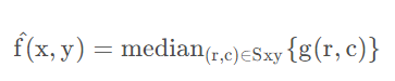
统计排序滤波器
统计排序滤波器是空间滤波器,其响应是基于滤波器邻域中的像素值的顺序,排序结果决定了滤波器的输出。
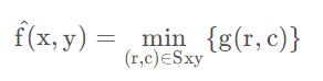
统计排序包括中值滤波器、最大值滤波器、最小值滤波器、中点滤波器和修正阿尔法均值滤波器。- 中值滤波器:用预定义的像素邻域中的灰度中值来代替像素的值,与线性平滑滤波器相比能有效地降低某些随机噪声,且模糊度要小得多。
-
最大值滤波器:用预定义的像素邻域中的灰度最大值来代替像素的值,可用于找到图像中的最亮点,或用于消弱与明亮区域相邻的暗色区域,也可以用来降低胡椒噪声。

-
最小值滤波器:用预定义的像素邻域中的灰度最小值来代替像素的值,可用于找到图像中的最暗点,或用于削弱与暗色区域相邻的明亮区域,也可以用来降低盐粒噪声。
- 中点滤波器:用预定义的像素邻域中的灰度的最大值与最小值的均值来代替像素的值,注意中点的取值与中值常常是不同的。中点滤波器是统计排序滤波器与平均滤波器的结合,适合处理随机分布的噪声,例如高斯噪声、均匀噪声。
示例程序:
""" 统计排序滤波器 """ import cv2 import matplotlib.pyplot as plt import numpy as np img = cv2.imread("../img/lena_noise.jpg", 0) img_h = img.shape[0] img_w = img.shape[1] m, n = 3, 3 kernalMean = np.ones((m, n), np.float32) # 生成盒式核 # 边缘填充 hPad = int((m - 1) / 2) wPad = int((n - 1) / 2) imgPad = np.pad(img.copy(), ((hPad, m - hPad - 1), (wPad, n - wPad - 1)), mode="edge") imgMedianFilter = np.zeros(img.shape) # 中值滤波器 imgMaxFilter = np.zeros(img.shape) # 最大值滤波器 imgMinFilter = np.zeros(img.shape) # 最小值滤波器 imgMiddleFilter = np.zeros(img.shape) # 中点滤波器 for i in range(img_h): for j in range(img_w): # # 1. 中值滤波器 (median filter) pad = imgPad[i:i + m, j:j + n] imgMedianFilter[i, j] = np.median(pad) # # 2. 最大值滤波器 (maximum filter) pad = imgPad[i:i + m, j:j + n] imgMaxFilter[i, j] = np.max(pad) # # 3. 最小值滤波器 (minimum filter) pad = imgPad[i:i + m, j:j + n] imgMinFilter[i, j] = np.min(pad) # # 4. 中点滤波器 (middle filter) pad = imgPad[i:i + m, j:j + n] imgMiddleFilter[i, j] = int(pad.max() / 2 + pad.min() / 2) plt.figure(figsize=(9, 7)) plt.subplot(221), plt.axis('off'), plt.title("median filter") plt.imshow(imgMedianFilter, cmap='gray', vmin=0, vmax=255) plt.subplot(222), plt.axis('off'), plt.title("maximum filter") plt.imshow(imgMaxFilter, cmap='gray', vmin=0, vmax=255) plt.subplot(223), plt.axis('off'), plt.title("minimum filter") plt.imshow(imgMinFilter, cmap='gray', vmin=0, vmax=255) plt.subplot(224), plt.axis('off'), plt.title("middle filter") plt.imshow(imgMiddleFilter, cmap='gray', vmin=0, vmax=255) plt.tight_layout() plt.show()- 1
- 2
- 3
- 4
- 5
- 6
- 7
- 8
- 9
- 10
- 11
- 12
- 13
- 14
- 15
- 16
- 17
- 18
- 19
- 20
- 21
- 22
- 23
- 24
- 25
- 26
- 27
- 28
- 29
- 30
- 31
- 32
- 33
- 34
- 35
- 36
- 37
- 38
- 39
- 40
- 41
- 42
- 43
- 44
- 45
- 46
- 47
- 48
- 49
- 50
- 51
- 52
- 53

原图添加的椒盐噪声,可以看到中值滤波滤除得较好。修正阿尔法均值滤波器
修正阿尔法均值滤波器也属于统计排序滤波器,其思想类似于比赛中去掉最高分和最低分后计算平均分。
其计算公式为:
d表示d个最低灰度值和d个最高灰度值,d 的取值范围是[0,mn/2−1]。选择d的大小对图像处理的效果影响很大,当 d=0 时简化为算术平均滤波器,当 d=mn/2−1 简化为中值滤波器。示例程序:
""" 修正阿尔法均值滤波器 """ import cv2 import matplotlib.pyplot as plt import numpy as np img = cv2.imread("../img/lena_noise.jpg", 0) img_h = img.shape[0] img_w = img.shape[1] m, n = 5, 5 kernalMean = np.ones((m, n), np.float32) # 生成盒式核 # 边缘填充 hPad = int((m - 1) / 2) wPad = int((n - 1) / 2) imgPad = np.pad(img.copy(), ((hPad, m - hPad - 1), (wPad, n - wPad - 1)), mode="edge") imgAlphaFilter0 = np.zeros(img.shape) imgAlphaFilter1 = np.zeros(img.shape) imgAlphaFilter2 = np.zeros(img.shape) for i in range(img_h): for j in range(img_w): # 邻域 m * n pad = imgPad[i:i + m, j:j + n] padSort = np.sort(pad.flatten()) # 对邻域像素按灰度值排序 d = 1 sumAlpha = np.sum(padSort[d:m * n - d - 1]) # 删除 d 个最大灰度值, d 个最小灰度值 imgAlphaFilter0[i, j] = sumAlpha / (m * n - 2 * d) # 对剩余像素进行算术平均 d = 2 sumAlpha = np.sum(padSort[d:m * n - d - 1]) imgAlphaFilter1[i, j] = sumAlpha / (m * n - 2 * d) d = 4 sumAlpha = np.sum(padSort[d:m * n - d - 1]) imgAlphaFilter2[i, j] = sumAlpha / (m * n - 2 * d) plt.figure(figsize=(9, 7)) plt.subplot(221), plt.axis('off'), plt.title("Original") plt.imshow(img, cmap='gray', vmin=0, vmax=255) plt.subplot(222), plt.axis('off'), plt.title("Modified alpha-mean(d=1)") plt.imshow(imgAlphaFilter0, cmap='gray', vmin=0, vmax=255) plt.subplot(223), plt.axis('off'), plt.title("Modified alpha-mean(d=2)") plt.imshow(imgAlphaFilter1, cmap='gray', vmin=0, vmax=255) plt.subplot(224), plt.axis('off'), plt.title("Modified alpha-mean(d=4)") plt.imshow(imgAlphaFilter2, cmap='gray', vmin=0, vmax=255) plt.tight_layout() plt.show()- 1
- 2
- 3
- 4
- 5
- 6
- 7
- 8
- 9
- 10
- 11
- 12
- 13
- 14
- 15
- 16
- 17
- 18
- 19
- 20
- 21
- 22
- 23
- 24
- 25
- 26
- 27
- 28
- 29
- 30
- 31
- 32
- 33
- 34
- 35
- 36
- 37
- 38
- 39
- 40
- 41
- 42
- 43
- 44
- 45
- 46
- 47
- 48
- 49
- 50
- 51
- 52

-
相关阅读:
SSTables和LSM-Tree
JavaSE学习----(八)常用类之String类
一些值得阅读的前端文章(不定期更新)
计算机毕业设计SSM成绩管理与学情分析系统【附源码数据库】
vscode 常用插件
鸿蒙HarmonyOS实战-ArkUI组件(Video)
LeetCode 1470. 重新排列数组 / 654. 最大二叉树 / 998. 最大二叉树 II
(Research)肝肿瘤免疫微环境亚型和中性粒细胞异质性
中小企业的公司财务管理系统
Detectron2环境配置加测试(Linux)
- 原文地址:https://blog.csdn.net/qq1198768105/article/details/126586908