【深度学习】图像分割概述

图像分割

与目标检测不同，语义分割可以识别并理解图像中每一个像素的内容：其语义区域的标注和预测是像素级的。与目标检测相比，语义分割中图像有关狗、猫和背景的标签，语义分割标注的像素级的边框显然更加精细。

本文主要梳理基于深度学习的图像分割方法。按照任务不同，可以将图像分割分为三类：语义分割、实例分割、全景分割。

语义分割： 语义分割是指将图像中的像素分类为语义类。属于特定类别的像素仅被分类到该类别，而不考虑其他信息或上下文。

实例分割： 实例分割模型根据“实例”而不是类别将像素分类。

全景分割： 全景分割是最新开发的分割任务，可以表示为语义分割和实例分割的组合，其中图像中对象的每个实例都被分离，并预测对象的身份。和实例分割的区别在于，将整个图像都进行分割。

1. 语义分割

1.1 U-Net原理与实现

可以按照以下思路进行理解：数据读取器DataLoader，网络Network，损失函数Loss Function，训练方法及优化器Train Setting。上述代码中，标签是RGB像素值，因此会出现预测的图像有不同的颜色出现。还有一种标签就是将像素值映射成类别值。

结合这张图可以理解怎么构造UNet网络。可以看出来，经过c1, c2, c3, c4, c5。图像的尺寸逐渐变小，尺寸变为16×16，这个过程成为Encode过程。为了进行像素级别的分类，采取的思路是，将编码的矩阵进行上采样，尺寸变大，并且和之前编码的尺寸相同的矩阵在通道方向进行叠加，如灰色箭头所示。进行若干次叠加，最后将其映射成概率值，进行像素级别上的分类。

1.1.1 DataLoader

transform=transforms.Compose([
    transforms.ToTensor()
])
class MyDataset(Dataset):
    def __init__(self,path):
        self.path=path
        self.name=os.listdir(os.path.join(path,'SegmentationClass'))

    def __len__(self):
        return len(self.name)      # 数据集的数量

    def __getitem__(self, index):
        segment_name=self.name[index]  #xx.png
        segment_path=os.path.join(self.path,'SegmentationClass',segment_name)
        print(segment_path)
        image_path=os.path.join(self.path,'JPEGImages',segment_name.replace('png','jpg'))
        segment_image=keep_image_size_open(segment_path)
        image=keep_image_size_open(image_path)
        return transform(image),transform(segment_image)
1
2
3
4
5
6
7
8
9
10
11
12
13
14
15
16
17
18
19

注意以下几点：图片的尺寸需要统一并将像素一一对应；图片和标签的数据类型与尺寸image shape = (n, c, h, w), label shape = (n, c, h, w) 。

1.1.2 Network

class UNet(nn.Module):
    def __init__(self):
        super(UNet, self).__init__()
        self.c1=Conv_Block(3,64)  # 卷积Block
        self.d1=DownSample(64)   
        self.c2=Conv_Block(64,128)
        self.d2=DownSample(128)
        self.c3=Conv_Block(128,256)
        self.d3=DownSample(256)
        self.c4=Conv_Block(256,512)
        self.d4=DownSample(512)
        self.c5=Conv_Block(512,1024)
        self.u1=UpSample(1024)
        self.c6=Conv_Block(1024,512)
        self.u2 = UpSample(512)
        self.c7 = Conv_Block(512, 256)
        self.u3 = UpSample(256)
        self.c8 = Conv_Block(256, 128)
        self.u4 = UpSample(128)
        self.c9 = Conv_Block(128, 64)
        self.out=nn.Conv2d(64,3,3,1,1)  # inc=64, outc=3 , kernal_size=3, stride=1, padding=1
        self.Th=nn.Sigmoid()

    def forward(self,x):
        R1=self.c1(x)
        # print('R1.shape:', R1.shape)  # 2*64*256*256
        R2=self.c2(self.d1(R1))
        # print('R2.shape:', R2.shape) # 2*128*128*128
        R3 = self.c3(self.d2(R2))
        # print('R3.shape:', R3.shape)  # 2*256*64*64
        R4 = self.c4(self.d3(R3))     
        # print('R4.shape:', R4.shape)  # 2*512*32*32
        R5 = self.c5(self.d4(R4))
        # print('R5.shape:', R5.shape)  # 2*1024*16*16
        O1 = self.c6(self.u1(R5,R4))  # 2*1024*16*16  （变化） cat 2*512*32*32   -> 2*512*32*32
        O2 = self.c7(self.u2(O1, R3)) # 2*512*32*32   （变化） cat 2*256*64*64   -> 2*256*64*64
        O3 = self.c8(self.u3(O2, R2)) # 2*256*64*64   （变化） cat 2*128*128*128 -> 2*128*128*128
        O4 = self.c9(self.u4(O3, R1)) # 2*128*128*128 （变化） cat 2*64*256*256  -> 2*64*256*256

        return self.Th(self.out(O4))  # 2*64*256*256 -> 2*3*256*256  -> sigmoid() 求了一个概率值
1
2
3
4
5
6
7
8
9
10
11
12
13
14
15
16
17
18
19
20
21
22
23
24
25
26
27
28
29
30
31
32
33
34
35
36
37
38
39
40

1.1.3 Train

net=UNet().to(device)
opt=optim.Adam(net.parameters())
loss_fun=nn.BCELoss()
while True:
    running_loss = 0.0
    print('Epoch {}/{}'.format(epoch, 10000))
    for i,(image,segment_image) in enumerate(data_loader):
        image, segment_image=image.to(device),segment_image.to(device)
        # print(torch.unique(segment_image))
        # print('type(segment_image):', type(segment_image), 
        # 'segment_image.shape: ', segment_image.shape, 'image.shape:', image.shape)    image.shape = [2, 3, 256, 256]  segment.shape = [2, 3, 256, 256]
        out_image=net(image) # out_image.shape = [2, 3, 256, 256]
        train_loss=loss_fun(out_image,segment_image)

        opt.zero_grad()
        train_loss.backward()
        opt.step()
        running_loss += train_loss.data.item()
        epoch_loss = running_loss / epoch

        if i%5==0:
            print(f'{epoch}-{i}-train_loss===>>{train_loss.item()}')

            if i%100==0:
                torch.save(net.state_dict(),weight_path)

                _image=image[0]
                _segment_image=segment_image[0]
                _out_image=out_image[0]
                print("++++++++++++++out_image:", _out_image)

                img=torch.stack([_image,_segment_image,_out_image],dim=0)
                save_image(img,f'{save_path}/{i}.png')

                writer.add_scalar('data/trainloss', epoch_loss, epoch)

                if epoch%1000 == 0:
                    torch.save(net, 'checkpoints/model_epoch_{}.pth'.format(epoch))
                    print('checkpoints/model_epoch_{}.pth saved!'.format(epoch))

                    epoch+=1
1
2
3
4
5
6
7
8
9
10
11
12
13
14
15
16
17
18
19
20
21
22
23
24
25
26
27
28
29
30
31
32
33
34
35
36
37
38
39
40
41

关于利用loss计算时， 要关注网络的输出和标签的形状。因为nn封装的loss计算模块，对out_image, segment_image 的形状有规定。

2. 实例分割

2.1 RCNN

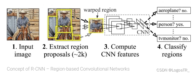
RCNN（Region with CNN feature）是卷积神经网络应用于目标检测问题的一个里程碑的飞跃。CNN具有良好的特征提取和分类性能，采用RegionProposal方法实现目标检测问题。算法可以分为三步：候选区域选择，CNN特征提取，分类与边界回归。

1. 候选区域选择：区域建议Region Proposal是一种传统的区域提取方法，基于启发式的区域提取方法，用的方法是选择性搜索（Selective Search, SS），查看现有的小区域，合并两个最有可能的区域，重复此步骤，直到图像合并为一个区域，最后输出候选区域。然后将根据建议提取的目标图像标准化，作为CNN的标准输入可以看作窗口通过滑动获得潜在的目标图像，在RCNN中一般Candidate选项为1k~2k，即可理解为将图片划分成1k~2k个网格，之后再对网格进行特征提取或卷积操作，这根据RCNN类算法下的分支来决定。然后基于就建议提取的目标图像将其标准化为CNN的标准输入。

2. CNN特征提取：标准卷积神经网络根据输入执行诸如卷积或池化的操作以获得固定维度输出。也就是说，在特征提取之后，特征映射被卷积和汇集以获得输出。

3. 分类与边界回归：实际上有两个子步骤，一个是对前一步的输出向量进行分类（分类器需要根据特征进行训练）; 第二种是通过边界回归框回归（缩写为bbox）获得精确的区域信息。其目的是准确定位和合并完成分类的预期目标，并避免多重检测。在分类器的选择中有支持向量机SVM，Softmax等等；边界回归有bbox回归，多任务损失函数边框回归等 。

R-CNN最大的问题有三：需要事先提取多个候选区域对应的图像。这一行为会占用大量的磁盘空间；针对传统的CNN来说，输入的map需要时固定尺寸的，而归一化过程中对图片产生的形变会导致图片大小改变，这对CNN的特征提取有致命的坏处；每个region proposal都需要进入CNN网络计算。进而会导致过多次的重复的相同的特征提取，这一举动会导致大大的计算浪费。

2.2 Faster R-CNN

Faster R-CNN是R-CNN架构的改进版本，具有两个阶段：

Region Proposal Network (RPN) 利用锚点和框回归机制不断接近Ground Truth 的框。

Fast R-CNN 利用RoIPool（兴趣区域池）从每个候选框中提取特征，并执行分类和边界框回归。RoIPool是用于从检测中的每个RoI提取小特征图的操作。

与rcnn最大的不同就在于RPN模块，极大减少计算量。

2.3 Mask R-CNN

Mask R-CNN原理与实现

Mask R-CNN是使用 Fast R-CNN构建的。Fast R-CNN对每个候选对象有2个输出: 一个类标签和一个边界框偏移，而Mask R-CNN设计了第三个分支输出对象掩码。额外的掩码输出不同于类和框输出，需要提取更精细的对象空间布局。

Mask R-CNN是 Fast R-CNN的扩展，其工作原理是添加一个用于预测对象掩码（感兴趣区域）的分支，与用于边界框识别的现有分支并行。

pytorch 实现mask rcnn

其他实现方法

DataLoader

import os
import numpy as np
import torch
from PIL import Image


class PennFudanDataset(torch.utils.data.Dataset):
    def __init__(self, root, transforms):
        self.root = root
        self.transforms = transforms
        # load all image files, sorting them to
        # ensure that they are aligned
        self.imgs = list(sorted(os.listdir(os.path.join(root, "PNGImages"))))
        self.masks = list(sorted(os.listdir(os.path.join(root, "PedMasks"))))
        
    def __getitem__(self, idx):
        # load images and masks
        img_path = os.path.join(self.root, "PNGImages", self.imgs[idx])
        mask_path = os.path.join(self.root, "PedMasks", self.masks[idx])
        img = Image.open(img_path).convert("RGB")
        # note that we haven't converted the mask to RGB,
        # because each color corresponds to a different instance
        # with 0 being background
        mask = Image.open(mask_path)
        # convert the PIL Image into a numpy array
        mask = np.array(mask)
        # instances are encoded as different colors
        obj_ids = np.unique(mask)
        # first id is the background, so remove it
        obj_ids = obj_ids[1:]

        # split the color-encoded mask into a set
        # of binary masks
        masks = mask == obj_ids[:, None, None]

        # get bounding box coordinates for each mask
        num_objs = len(obj_ids)
        boxes = []
        for i in range(num_objs):
            pos = np.where(masks[i])
            xmin = np.min(pos[1])
            xmax = np.max(pos[1])
            ymin = np.min(pos[0])
            ymax = np.max(pos[0])
            boxes.append([xmin, ymin, xmax, ymax])

        # convert everything into a torch.Tensor
        boxes = torch.as_tensor(boxes, dtype=torch.float32)
        # there is only one class
        labels = torch.ones((num_objs,), dtype=torch.int64)
        masks = torch.as_tensor(masks, dtype=torch.uint8)

        image_id = torch.tensor([idx])
        area = (boxes[:, 3] - boxes[:, 1]) * (boxes[:, 2] - boxes[:, 0])
        # suppose all instances are not crowd
        iscrowd = torch.zeros((num_objs,), dtype=torch.int64)

        target = {}
        target["boxes"] = boxes
        target["labels"] = labels
        target["masks"] = masks
        target["image_id"] = image_id
        target["area"] = area
        target["iscrowd"] = iscrowd

        if self.transforms is not None:
            img, target = self.transforms(img, target)

        return img, target

    def __len__(self):
        return len(self.imgs)
1
2
3
4
5
6
7
8
9
10
11
12
13
14
15
16
17
18
19
20
21
22
23
24
25
26
27
28
29
30
31
32
33
34
35
36
37
38
39
40
41
42
43
44
45
46
47
48
49
50
51
52
53
54
55
56
57
58
59
60
61
62
63
64
65
66
67
68
69
70
71
72

• image: a PIL Image of size (H, W)
• target: a dict containing the following fields
  • boxes (FloatTensor[N, 4]): the coordinates of the N bounding boxes in [x0, y0, x1, y1] format, ranging from 0 to W and 0 to H
  • labels (Int64Tensor[N]): the label for each bounding box. 0 represents always the background class.
  • image_id (Int64Tensor[1]): an image identifier. It should be unique between all the images in the dataset, and is used during evaluation
  • area (Tensor[N]): The area of the bounding box. This is used during evaluation with the COCO metric, to separate the metric scores between small, medium and large boxes.
  • iscrowd (UInt8Tensor[N]): instances with iscrowd=True will be ignored during evaluation.
  • (optionally) masks (UInt8Tensor[N, H, W]): The segmentation masks for each one of the objects

Network

import torchvision
from torchvision.models.detection.faster_rcnn import FastRCNNPredictor
from torchvision.models.detection.mask_rcnn import MaskRCNNPredictor


def get_model_instance_segmentation(num_classes):
    # load an instance segmentation model pre-trained on COCO
    model = torchvision.models.detection.maskrcnn_resnet50_fpn(weights="DEFAULT")

    # get number of input features for the classifier
    in_features = model.roi_heads.box_predictor.cls_score.in_features
    # replace the pre-trained head with a new one
    model.roi_heads.box_predictor = FastRCNNPredictor(in_features, num_classes)

    # now get the number of input features for the mask classifier
    in_features_mask = model.roi_heads.mask_predictor.conv5_mask.in_channels
    hidden_layer = 256
    # and replace the mask predictor with a new one
    model.roi_heads.mask_predictor = MaskRCNNPredictor(in_features_mask,
                                                       hidden_layer,
                                                       num_classes)

    return model
1
2
3
4
5
6
7
8
9
10
11
12
13
14
15
16
17
18
19
20
21
22
23

Train

from engine import train_one_epoch, evaluate
import utils

def main():
    # train on the GPU or on the CPU, if a GPU is not available
    device = torch.device('cuda') if torch.cuda.is_available() else torch.device('cpu')
    
    # our dataset has two classes only - background and person
    num_classes = 2
    # use our dataset and defined transformations
    dataset = PennFudanDataset('PennFudanPed', get_transform(train=True))
    dataset_test = PennFudanDataset('PennFudanPed', get_transform(train=False))

    # split the dataset in train and test set
    indices = torch.randperm(len(dataset)).tolist()
    dataset = torch.utils.data.Subset(dataset, indices[:-50])
    dataset_test = torch.utils.data.Subset(dataset_test, indices[-50:])

    # define training and validation data loaders
    data_loader = torch.utils.data.DataLoader(
        dataset, batch_size=2, shuffle=True, num_workers=4,
        collate_fn=utils.collate_fn)

    data_loader_test = torch.utils.data.DataLoader(
        dataset_test, batch_size=1, shuffle=False, num_workers=4,
        collate_fn=utils.collate_fn)

    # get the model using our helper function
    model = get_model_instance_segmentation(num_classes)

    # move model to the right device
    model.to(device)

    # construct an optimizer
    params = [p for p in model.parameters() if p.requires_grad]
    optimizer = torch.optim.SGD(params, lr=0.005,
                                momentum=0.9, weight_decay=0.0005)
    # and a learning rate scheduler
    lr_scheduler = torch.optim.lr_scheduler.StepLR(optimizer,
                                                   step_size=3,
                                                   gamma=0.1)

    # let's train it for 10 epochs
    num_epochs = 10

    for epoch in range(num_epochs):
        # train for one epoch, printing every 10 iterations
        train_one_epoch(model, optimizer, data_loader, device, epoch, print_freq=10)
        # update the learning rate
        lr_scheduler.step()
        # evaluate on the test dataset
        evaluate(model, data_loader_test, device=device)

    print("That's it!")
1
2
3
4
5
6
7
8
9
10
11
12
13
14
15
16
17
18
19
20
21
22
23
24
25
26
27
28
29
30
31
32
33
34
35
36
37
38
39
40
41
42
43
44
45
46
47
48
49
50
51
52
53
54

上述代码完整版参考此链接

差异检测

和语义分割任务类似，在像素级别上进行分类，只不过差异检测的类别比较特殊，仅含两类：像素有变化，像素无变化。