多目标进化算法详细讲解及代码实现（样例：MOEA/D、NSGA-Ⅱ求解多目标（柔性）作业车间调度问题）

注：文中涉及到的所有子目标几乎都为最小化

1 多目标问题的数学形式

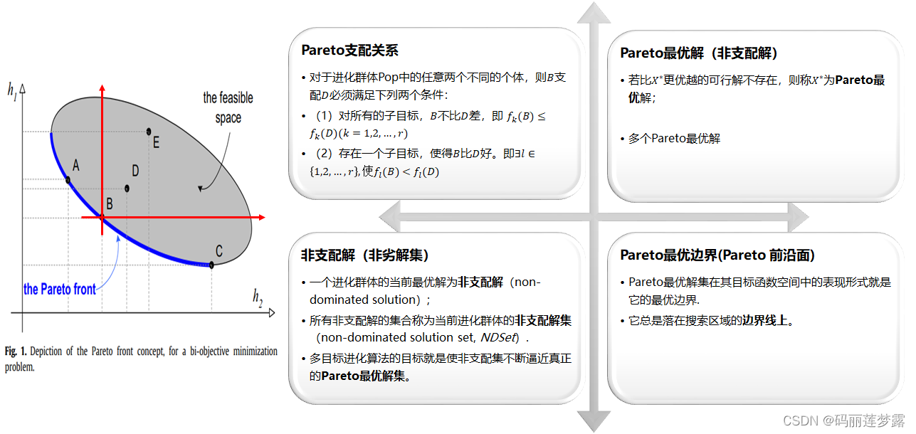
2 多目标的相关理论基础

3 基于分解的多目标进化算法

基本思路：在给定权重偏好或者参考点信息的情况下，分解方法通过线性或者非线性方式将原多目标问题各个目标进行聚合，得到单目标优化问题。在对各个部分进行详细讲解之前，首先放上基于MOEA/D的一个基本流程做框架演示，如下图：

3.1 权重向量生成方法

基于分解的多目标进化算法首先需要产生一组均匀分布的权重向量。

参考文献：K. Li, K. Deb, Q. Zhang and S. Kwong, "An Evolutionary Many-Objective Optimization Algorithm Based on Dominance and Decomposition," in IEEE Transactions on Evolutionary Computation, vol. 19, no. 5, pp. 694-716, Oct. 2015, doi: 10.1109/TEVC.2014.2373386.

3.1.1 Systematic approach

这个方法中，权重向量基于单位超平面产生，且总个数为 $C_{m-1}^{H+m-1}$ $N=C^{m-1}_{H+m-1}$ ,其中，m是目标的个数，H（H>=m）是多目标问题中每个维度的坐标轴的间隔数量。下图展示了一个3目标，各目标维度4等分的案例。

3.1.2 two-layer weight vector generation method（two-layer权重向量生成方法）

3.1.1的方法在低维度中可以使用，但在高维目标空间中,权重向量的数量特别多，例如，目标数量为7个时，我们令H=7，那么以上面的方法权重向量的组合数为 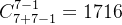$C^{7-1}_{7+7-1}=1716$ 组，这显然加剧了多目标进化算法的计算负担；另一方面，如果我们简单地降低H（例如设置H

two-layer权重向量生成方法将权重向量分为两层：边界层（ $B=\left \{ b_{1},...,b_{N_{1}} \right \}$ ）和内部层 $I=\left \{ i_{1},...,i_{N_{2}} \right \}$ ,其中 $N_{1}+N_{2}=N$ ,N为种群数量。首先，边界层和内部层根据3.1.1的方法生成不同的H值对应的权重向量，然后通过下式进行坐标转换来缩小内层权重向量 $i^{k}=(i_{1}^{k},...,i_{m}^{k})$ (m个目标)的坐标：

边界层的权重向量根据上述方法得到，通常，我们取 $\tau =0.5$ .

3.2 聚合函数

将多个目标聚合的方式有多种，包括线性的多目标加权或者非线性聚合方法，下面介绍分解策略中三类常用的聚合函数。

3.2.1 权重聚合方法

这是一种线性聚合方法，下式 $\lambda$ 为权重向量， $f_{i}(x)$ 表示第个目标。权重聚合方法的等值线为一族与方向向量垂直的平行直线。

注：等值线表示在线上的所有可行解的目标函数值都相等。

由下面两个图可以见得，当真实的Pareto前沿面为凸状时，单个最优等值线与Pareto前沿面相交于一个切点，即权重聚合方法的最优解。当真实Pareto前沿面为凹状（右图，两图的优化目标都是最小化），权重聚合函数的最优解位于Pareto面的边缘区域，这是因为位于Pareto面的中间部分的解具有较差的适应度值。因此，权重聚合方法不能很好的处理真实Pareto面为凹状的问题。

3.2.2 切比雪夫的方法(Tchebycheff approach)

切比雪夫方法是一种非线性聚合方法，与权重聚合方法的加权和不同，在计算目标函数值前，需要计算种群中截至目前为止的各目标取得的最小值作为参考点 $Z^{*}$ （作为一个理想目标值，真实场景下可能不存在）。目标函数值为个体的各个目标与其目标参考值（该目标截至目前为止发现的最小值）的加权距离（即 $\lambda _{i}\left | f_{i}(x)-Z_{i}^{*} \right |$ ）的最大值，明显只知，切比雪夫的等值线方向呈直角锯齿状。

为什么是直角锯齿状？（个人理解，可能表述不太好，见谅）

当在 $f_{1}$ 上取加权距离为目标函数值时，

具有与 $f_{1}$ 相同的目标值

且 $f_{2}$ 上加权距离和（ $\lambda _{i}\left | f_{i}(x)-Z_{i}^{*} \right |$ ）小于 $f_{1}$ 的加权距离和

那么符合这个要求的可行解个体在与 $f_{1}$ 坐标轴垂直的线上.

同理，在 $f_{2}$ 上取加权距离为目标函数值时，可行解个体则在与 $f_{2}$ 坐标轴垂直的线上，因而，当 $f_{1}$ 上取加权距离为目标函数值== $f_{2}$ 上取加权距离为目标函数值，则易于理解为何呈直角锯齿状。

直观上看，在连续Pareto面情形下，切比雪夫子问题的最优解为方向向量（与权重向量垂直）与Pareto面的交点。在非连续Pareto面情形下，对应不同权重向量的子问题可能具有相同的最优解，这是因为方向向量与Pareto面没有交点。在处理高维问题时，切比雪夫方法限制收敛接受区域，因而能更好的保证种群的收敛性。


def Tchebycheff(x, z, lambd):
    '''
    :param x: Popi
    :param z: the reference point
    :param lambd: a weight vector
    :return: Tchebycheff objective
    '''
    Gte = []
    for i in range(len(x.fitness)):
        Gte.append(np.abs(x.fitness[i]-z[i]) * lambd[i])
    return np.max(Gte)

3.2.3 边界交叉方法（boundary intersection approach, BI）

交叉边界法（BI）主要是为连续多目标优化问题设计的，可以用于处理非凸Pareto前沿面的多目标优化问题。其中等式约束 $Z^{*}-F(x)=\lambda d$ 是为了保证F(x)位于权重向量的方向上，算法通过减小d来逐渐逼近PF。

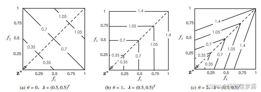
基于惩罚的交叉边界法放宽了对可行解的要求，但加入了一个惩罚措施，即如果不在权重向量方向上就要接受惩罚，距离权重向量越远，惩罚越厉害，惩罚力度通过 $\theta$ 来调节，于是基于惩罚的交叉边界法的等值线可见第3副图。

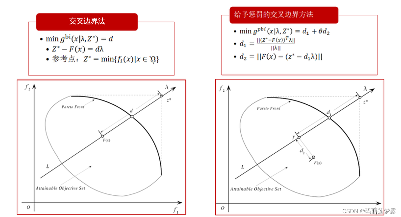
3.3 基于分解的MOEA算法：MOEA/D

参考文献：Q. Zhang and H. Li, "MOEA/D: A Multiobjective Evolutionary Algorithm Based on Decomposition," in IEEE Transactions on Evolutionary Computation, vol. 11, no. 6, pp. 712-731, Dec. 2007, doi: 10.1109/TEVC.2007.892759.

3.3.1 输入/输出

输入：多目标优化问题、停止准则、优化目标数N、均匀分布的权重向量、每个权重向量邻居数T

输出：非支配解集EP

伪代码及算法流程步骤如下：

3.3.2 MOEA/D主程序


    def main(self):
        # ----------------------------------Initialization---------------------------------
        # to obtain Populations and weight vectors
        if self.means_m>1:      # Used to determine whether the machine is flexible
            self.random_initial()       # random Initial
            self.GS_initial()           # Globel Initial
            self.LS_initial()           # Local Initial
        else:
            self.random_initial_0()     # if the flexibility of machine is None. use random Initial
        B=Neighbor(self._lambda,self.T)     # work out the T closest weight vectors to each weight vector
        EP=[]   # EP is used to store non-dominated solutions found during the search
        # ----------------------------------Iteration---------------------------------
        for gi in range(self.gene_size):
            # Adaptive operator rate
            self.pc = self.pc_max - ((self.pc_max - self.pc_min) / self.gene_size) * gi
            self.pm = self.pm_max - ((self.pm_max - self.pm_min) / self.gene_size) * gi
            for i in range(self.Pop_size):
                # Randomly select two indexes k,l from B(i)
                j = random.randint(0, self.T- 1)
                k = random.randint(0, self.T- 1)
                # generate new solution from pop[j] and pop[k] by using genetic operators
                if self.means_m>1:
                    pop1,pop2=self.operator_Flexible(self.Pop[B[i][j]],self.Pop[B[i][k]])
                else:
                    pop1, pop2 = self.operator_NoFlexible(self.Pop[B[i][j]], self.Pop[B[i][k]])
                if Dominate(pop1,pop2):
                    y=pop1
                else:
                    y=pop2
                # update of the reference point z
                for zi in range(len(self._z)):
                    if self._z[zi]>y.fitness[zi]:
                        self._z[zi]=y.fitness[zi]
                # update of Neighboring solutions
                for bi in range(len(B[i])):
                    Ta = Tchebycheff(self.Pop[B[i][bi]], self._z, self._lambda[B[i][bi]])
                    Tb = Tchebycheff(y, self._z, self._lambda[B[i][bi]])
                    if Tb < Ta:
                        self.Pop[B[i][j]] = y
                # Update of EP
                if EP==[]:
                    EP.append(y)
                else:
                    dominateY = False  # 是否有支配Y的解
                    _remove = []  # Remove from EP all the vectors dominated by y
                    for ei in range(len(EP)):
                        if Dominate(y, EP[ei]):
                            _remove.append(EP[ei])
                        elif Dominate(EP[ei], y):
                            dominateY = True
                            break
                    # add y to EP if no vectors in EP dominated y
                    if not dominateY:
                        EP.append(y)
                        for j in range(len(_remove)):
                            EP.remove(_remove[j])
        Plot_NonDominatedSet(EP)
        return EP

4 基于Pareto的MOEA

步骤1：产生初始化种群P；

步骤2：选择某个进化算法（如遗传算法）对P执行进化操作（如交叉、变异和选择），得到新的进化种群R；

步骤3：采用某种策略构造P∪R的非支配集NDSet,一般情况下在设计算法时已经设置了非支配集的大小（如N）。

步骤4：若当前非支配集NDSet的大小大于或小于N时，需要按照某种策略对NDSet进行调整，调整时一方面使NDSet满足大小要求，同时也必须使NDSet满足分布性要求；

步骤5：判断终止条件，否则，迭代。

下面以个人所写的NSGA-Ⅱ的主程序为例，以作展示：


    def NSGA_main(self):
        # ----------------------------------Initialization---------------------------------
        self.Pop=[]
        if self.means_m > 1:  # Used to determine whether the machine is flexible
            self.random_initial()  # random Initial
            self.GS_initial()  # Globel Initial
            self.LS_initial()  # Local Initial
        else:
            self.random_initial_0()  # if the flexibility of machine is None. use random Initial
        # ----------------------------------Iteration---------------------------------
        for i in range(self.gene_size):
            new_pop=self.offspring_Population()     # use crossover and mutation to create a new population
            R_pop=self.Pop+new_pop # combine parent and offspring population
            NDSet=fast_non_dominated_sort(R_pop)    # all nondominated fronts of R_pop
            j=0
            self.Pop=[]
            while len(self.Pop)+len(NDSet[j])<=self.Pop_size:   # until parent population is filled
                self.Pop.extend(NDSet[j])
                j+=1
            if len(self.Pop)
                Ds=crowding_distance(copy.copy(NDSet[j]))       # calcalted crowding-distance
                k = 0
                while len(self.Pop) < self.Pop_size:
                    self.Pop.append(NDSet[j][Ds[k]])
                    k += 1
        EP=fast_non_dominated_sort(self.Pop)[0]
        return EP

决定基于Pareto的MOEA的关键点在于：

（1）如何选择构造非支配集的方法

（2）采用什么策略来调整非支配集的大小

（3）如何保持非支配集的分布性

最具代表性的基于支配的MOEA是：NSGA-Ⅱ，其算法流程如下：

5 求解多目标（柔性）作业车间调度问题

5.1 问题描述

详细的问题描述可见之前我之前的博文，不同的调度的目标在完工时间最小的基础上增加了最小化最大机器负荷和最小化机器总负荷。

用python实现改遗传算法解柔性作业车间调度问题的编码和初始化_码丽莲梦露的博客-CSDN博客_遗传算法车间调度编码

5.2 多目标算法代码架构

完整代码已上传至个人Github，可供大家参考：Aihong-Sun/MOEA-D-and-NSGA--for-FJSP: this repo has use MOEA/D and NSGA-Ⅱ to solve multi-objective FJSP problem (github.com)

Env_JSP_FJSP：（用于搭建作业车间/柔性作业车间的环境）

（1）Job.py

（2）Machine.py

（3）Job_Shop.py

Algorithms:

（1）Popi.py （一个个体，用于保存一个可行解的各种特征）

（2）utils.py （包含一个多目标的通用工具算子）

（3）Algorithms.py (包含MOEA/D和NSGA两种算法)

（4）Params.py (包含算法及问题的相关参数)

5.3参数设置

运行规模及相关参数设置如下，运行次数为1：


def get_args(n,m,PT,MT,ni,means_m=1):
    parser = argparse.ArgumentParser()
    # params for FJSPF:
    parser.add_argument('--n', default=n, type=int, help='job number')
    parser.add_argument('--m', default=m, type=int, help='Machine number')
    parser.add_argument('--O_num', default=ni, type=list, help='Operation number of each job')
    parser.add_argument('--Processing_Machine', default=MT, type=list, help='processing machine of operations')
    parser.add_argument('--Processing_Time', default=PT, type=list, help='fuzzy processing machine of operations')
    parser.add_argument('--means_m', default=means_m, type=float, help='avaliable machine')
 
    # Params for Algorithms
    parser.add_argument('--pop_size', default=100, type=int, help='Population size of the genetic algorithm')
    parser.add_argument('--gene_size', default=100, type=int, help='generation size of the genetic algorithm')
    parser.add_argument('--pc_max', default=0.8, type=float, help='Crossover rate')
    parser.add_argument('--pm_max', default=0.05, type=float, help='mutation rate')
    parser.add_argument('--pc_min', default=0.7, type=float, help='Crossover rate')
    parser.add_argument('--pm_min', default=0.01, type=float, help='mutation rate')
    parser.add_argument('--p_GS', default=0, type=float, help='globel initial rate')
    parser.add_argument('--p_LS', default=0, type=float, help='Local initial rate')
    parser.add_argument('--p_RS', default=1, type=float, help='random initial rate')
    parser.add_argument('--T', default=10, type=int, help='the number of the weight vectors in the neighborhood of each weight vector')
    parser.add_argument('--H', default=16, type=int,
                        help='the number of divisions considered along each objective coordinate')
    parser.add_argument('--N_elite', default=2, type=int, help='Elite number')
    args = parser.parse_args()
    return args

5.4 结果演示

注1：求解结果有待进一步改进，此处仅用作算法演示，具体改进可以相互交流。

注2：下面图很多，只是算例不同，至于为什么选那几个图，是因为我觉得看着好看，哈哈哈哈，所有结果可见上面提供的Github中，每个算例的结果都有。

5.4.1 两目标

5.4.2 三目标

此篇博文的完整代码已上传至个人Github，可供大家参考：Aihong-Sun/MOEA-D-and-NSGA--for-FJSP: this repo has use MOEA/D and NSGA-Ⅱ to solve multi-objective FJSP problem (github.com)

相关阅读:
Docker的安装
 【GNN】【ICML2019】Position-aware GraphNeural Networks
Spring中的面试题01
ADC采集到的数值和电压值、频率有什么联系？
使用 Docker 部署 instantbox 轻量级 Linux 系统
 【VScode】保存文件自动按照eslint规范格式化
 SPL工业智能：发现时序数据的异常
 Uniapp导出的iOS应用上架详解
 网络基础-4
LoggerMessageAttribute 高性能的日志记录
原文地址：https://blog.csdn.net/crazy_girl_me/article/details/125594561