一、 导入数据

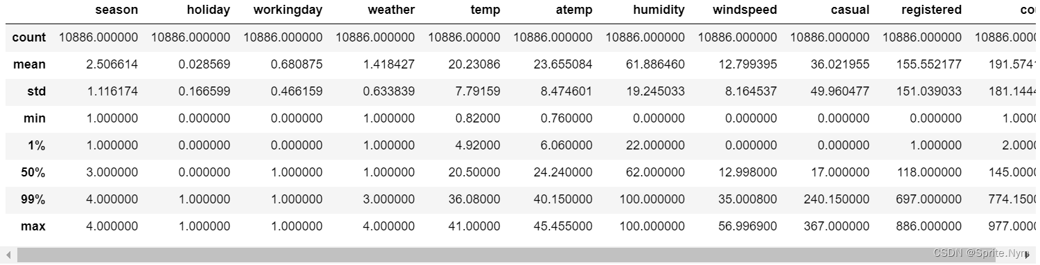
import numpy as np
import pandas as pd
import matplotlib.pyplot as plt
import seaborn as sns
sns.set()
%config InlineBackend.figure_format = 'svg'

bike_df0 = pd.read_csv('data/bike/train.csv')
bike_df0.info()
"""

RangeIndex: 10886 entries, 0 to 10885
Data columns (total 12 columns):
 #   Column      Non-Null Count  Dtype  
---  ------      --------------  -----  
 0   datetime    10886 non-null  object 
 1   season      10886 non-null  int64  
 2   holiday     10886 non-null  int64  
 3   workingday  10886 non-null  int64  
 4   weather     10886 non-null  int64  
 5   temp        10886 non-null  float64
 6   atemp       10886 non-null  float64
 7   humidity    10886 non-null  int64  
 8   windspeed   10886 non-null  float64
 9   casual      10886 non-null  int64  
 10  registered  10886 non-null  int64  
 11  count       10886 non-null  int64  
dtypes: float64(3), int64(8), object(1)
memory usage: 1020.7+ KB
"""

bike_df0.describe([0.01, 0.99])
1
2
3
4
5
6
7
8
9
10
11
12
13
14
15
16
17
18
19
20
21
22
23
24
25
26
27
28
29
30
31
32

二、 特征工程

2.1 类型转换

bike_df1 = bike_df0.copy()

def transform_datetime(df):
    # 将datetime处理成datetime类型
    df.datetime = pd.to_datetime(df.datetime)
    # 分别得到year、hour特征
    df['year'] = df.datetime.dt.year
    df['hour'] = df.datetime.dt.hour
    # 原来的datetime抛弃
    df.drop(columns=['datetime'], inplace=True)

transform_datetime(bike_df1)
1
2
3
4
5
6
7
8
9
10
11
12

2.2 特征筛选

# 查看相关系数
plt.figure(figsize=(12, 8))
sns.heatmap(bike_df1.corr(), vmin=-1, cmap=plt.cm.coolwarm, annot=True)
1
2
3

# 丢弃atemp列、holiday列、windspeed列和count列
bike_df1.drop(columns=['atemp', 'holiday', 'windspeed', 'count'], inplace=True)
1
2

2.3 异常值处理

# 画图查看hour列、temp列、humidity列与count的关系
def show_img(df, col_name, value_name):
    temp = pd.pivot_table(df, index=[col_name], values=[value_name], aggfunc='mean')
    plt.figure(figsize=(6,4))
    sns.lineplot(
        x=col_name, 
        y=value_name,
        data=temp
    )
    plt.title(f'{col_name}-{value_name}')
    plt.show()
    
for col in ['hour', 'humidity', 'temp']:
    for value in ['casual', 'registered']:
        show_img(bike_df1, col, value)
1
2
3
4
5
6
7
8
9
10
11
12
13
14
15

从上图可以看出，湿度<20和>20，数据表现完全不同，认定湿度<20的样本为异常值，排除。另外温度低、中、高的数据表现也不同，考虑分成三个训练集去建模预测，最后整合。

# 处理hour
# 再次画图查看hour列
hour = pd.pivot_table(bike_df1, index=['hour'], values=['registered'])
sns.barplot(x=hour.index, y=hour['registered'])
1
2
3
4

这里尝试分箱，效果不好，放弃分箱。

# 处理humidity 认定humidity < 20的为异常数据，丢弃
def drop_data(df, col, tol):
    df.drop(index=df[df[col]<tol].index, inplace=True)
drop_data(bike_df1, 'humidity', 20)

# 处理temp
# 认定3摄氏度以下为异常数据，删除
drop_data(bike_df1, 'temp', 3)

# 尝试将温度拆分成3段来建模预测，但后续效果不好
# def split_df(df, col_name, bins):
#     return [df[(bins[i] <= df[col_name]) & (df[col_name] < bins[i+1])] for i in range(len(bins)-1)]
# df_list = split_df(bike_df1, 'temp', [0, 32, 37, 50])
1
2
3
4
5
6
7
8
9
10
11
12
13

2.4 类别特征转哑变量

bike_df1['season'] = bike_df1['season'].map({1: 'spring', 2: 'summer', 3: 'fall', 4: 'winter'})
bike_df1['weather'] = bike_df1['weather'].map({1: 'clear', 2: 'cloudy', 3: 'light_rain', 4: 'heavy_rain'})
bike_df1['workingday'] = bike_df1['workingday'].map({0: 'no_workingday', 1: 'is_workingday'})

def to_dummies(df, cols):
    return pd.concat([pd.get_dummies(df[col]) for col in cols] + [df.drop(columns=cols)], axis=1)

bike_df2 = to_dummies(bike_df1, ['season', 'weather', 'workingday', 'year'])
1
2
3
4
5
6
7
8

三、建模

from xgboost import XGBRegressor
from catboost import CatBoostRegressor
from sklearn.ensemble import RandomForestRegressor, StackingRegressor, VotingRegressor
from sklearn.svm import SVR
from sklearn.neighbors import KNeighborsRegressor
from sklearn.model_selection import train_test_split
from sklearn.model_selection import GridSearchCV, cross_val_score

X_train, X_test, y_train, y_test = train_test_split(bike_df2.drop(columns=['casual', 'registered']), bike_df2[['casual', 'registered']], test_size=0.2)

# 定义一个简单的试探建模效果的函数
def easy_try(model, X_train, X_test, y_train, y_test):
    model.fit(X_train, y_train['casual'])
    print('casual', model.score(X_test, y_test['casual']))
    model.fit(X_train, y_train['registered'])
    print('registered', model.score(X_test, y_test['registered']))
1
2
3
4
5
6
7
8
9
10
11
12
13
14
15
16

3.1 XGB

%%time
easy_try(XGBRegressor(n_estimators=10), X_train, X_test, y_train, y_test)

# XGB支持多标签建模预测，这里就不区分casual和registered了
# 多次调参以使预测结果不要出现负数
xgb = XGBRegressor(n_estimators=14, max_depth=10, reg_lambda=10)
xgb.fit(X_train, y_train)
# 查看R²值
print(xgb.score(X_test, y_test)) # 0.9059309080369857
# 查看预测值是否出现负数，如果出现了能否接受
pd.DataFrame(xgb.predict(X_test)).describe()
1
2
3
4
5
6
7
8
9
10
11

3.2 随机森林

%%time
easy_try(RandomForestRegressor(), X_train, X_test, y_train, y_test)
"""
casual 0.8873701620424612
registered 0.9220132387157473
CPU times: total: 4.84 s
Wall time: 4.47 s
"""
1
2
3
4
5
6
7
8

3.3 CatBoost

%%time
easy_try(CatBoostRegressor(), X_train, X_test, y_train, y_test)
"""
casual 0.8942355038852897
registered 0.9379193613461692
CPU times: total: 27.9 s
Wall time: 5.22 s
"""

# 和XGB一样调参防止负数
cbr = CatBoostRegressor(iterations=1000, depth=10, loss_function='Poisson')
cbr.fit(X_train, y_train['registered'])
# 查看R²值
print(cbr.score(X_test, y_test['registered'])) # 0.9377051781734137
# 查看是否有负数
pd.DataFrame(cbr.predict(X_test)).describe()
1
2
3
4
5
6
7
8
9
10
11
12
13
14
15
16

3.4 其他

svm、knn尝试过，效果不好。

stacking和voting效果无明显提升。

四、预测

test_df0 = pd.read_csv('data/bike/test.csv')
test_df1 = test_df0.copy()
test_df1.describe([0.01, 0.99])
1
2
3

test_df1.head()
1

# 时间做类型转换
transform_datetime(test_df1)

# 丢弃不需要的特征
test_df1.drop(columns=['atemp', 'holiday', 'windspeed'], inplace=True)

# 处理类别特征成哑变量
test_df1['season'] = test_df1['season'].map({1: 'spring', 2: 'summer', 3: 'fall', 4: 'winter'})
test_df1['weather'] = test_df1['weather'].map({1: 'clear', 2: 'cloudy', 3: 'light_rain', 4: 'heavy_rain'})
test_df1['workingday'] = test_df1['workingday'].map({0: 'no_workingday', 1: 'is_workingday'})

test_df2 = to_dummies(test_df1, ['season', 'weather', 'workingday', 'year'])

# 定义一个预测函数
def bike_predict(model, train_df, test_df, target_list):
    result = [test_df]
    for target in target_list:
        model.fit(train_df.drop(columns=target_list), train_df[target])
        result.append(pd.DataFrame(model.predict(test_df).reshape(-1,1)).rename(columns={0:target}))
    
    return pd.concat(result, axis=1) 

# 使用XGB预测
result_df1 = bike_predict(XGBRegressor(n_estimators=14, max_depth=10, reg_lambda=10), bike_df2, test_df2, ['casual', 'registered'])

# 使用CatBoost预测
# result_df1 = bike_predict(CatBoostRegressor(iterations=1000, depth=10, loss_function='Poisson'), bike_df2, test_df2, ['casual', 'registered'])

# 检查有无负数，负数能否接受
result_df1[['casual', 'registered']].describe()
1
2
3
4
5
6
7
8
9
10
11
12
13
14
15
16
17
18
19
20
21
22
23
24
25
26
27
28
29
30

# 后续拼接处理
result_df2 = pd.concat([test_df0[['datetime']], result_df1], axis=1)
result_df2['count'] = result_df2['casual'] + result_df2['registered']
result_df2['count'] = np.round(result_df2['count'].map(lambda x: 0 if x < 0 else x))
result_df2.set_index('datetime', inplace=True)
result_df2['count'].to_csv('data/bike/s.csv')
1
2
3
4
5
6

五、提交效果

由于比赛已经结束，成绩无法在分数板上显示。