预备知识
- import tensorflow as tf
- import numpy as np
- import matplotlib.pyplot as plt
- import random
- import pandas as pd
- plt.rcParams['font.sans-serif']=['SimHei'] #用来正常显示中文标签
- plt.rcParams['axes.unicode_minus']=False # 正常显示负号
tf.where()
tf.where(条件语句,真返回值,假返回值)
- a = tf.constant([1,2,3,1,1])
- b = tf.constant([0,1,3,4,5])
- c = tf.where(tf.greater(a,b),a,b) # 若a > b ,则返回a对应位置元素,否则返回b对应位置元素
- print(c)
tf.Tensor([1 2 3 4 5], shape=(5,), dtype=int32)np.random.RandomState.rand()
返回一个[0,1)之间的随机数
np.random.RandomState.rand(维度)
若参数 维度 为空,则返回一个0~1之间的标量
- rdm = np.random.RandomState(seed = 1) # seed=常数 每次产生的随机数相同
- a = rdm.rand() # 返回一个随机标量
- b = rdm.rand(2,3) # 返回维度为二行三列随机数矩阵(第一个维度两个元素,第二个维度三个元素)
- print("a:",a)
- print("b:",b)
- a: 0.417022004702574
- b: [[7.20324493e-01 1.14374817e-04 3.02332573e-01]
- [1.46755891e-01 9.23385948e-02 1.86260211e-01]]
np.vstack()
将两个数组按垂直方向叠加
np.vstack(数组1,数组2)
- a = np.array([1,2,3])
- b = np.array([3,3,3])
- c = np.vstack((a,b))
- print(c)
- [[1 2 3]
- [3 3 3]]
np.mgrid[] .ravel() np.c_[]
三个一起使用,生成网格坐标点
np.mgrid[]
np.mgrid[起始值:结束值:步长,起始值:结束值:步长,……]
x.ravel()
将x变为一维数组
np.c_[]
np.c_[数组1,数组2,……]
使返回的间隔数值点配对
- # 生成等间隔数值点
- x, y = np.mgrid[1:3:1, 2:4:0.5]
- # 将x, y拉直,并合并配对为二维张量,生成二维坐标点
- grid = np.c_[x.ravel(), y.ravel()]
- print("x:\n", x)
- print("y:\n", y)
- print("x.ravel():\n", x.ravel())
- print("y.ravel():\n", y.ravel())
- print('grid:\n', grid)
- x:
- [[1. 1. 1. 1.]
- [2. 2. 2. 2.]]
- y:
- [[2. 2.5 3. 3.5]
- [2. 2.5 3. 3.5]]
- x.ravel():
- [1. 1. 1. 1. 2. 2. 2. 2.]
- y.ravel():
- [2. 2.5 3. 3.5 2. 2.5 3. 3.5]
- grid:
- [[1. 2. ]
- [1. 2.5]
- [1. 3. ]
- [1. 3.5]
- [2. 2. ]
- [2. 2.5]
- [2. 3. ]
- [2. 3.5]]

神经网络(NN)复杂度
NN复杂度:多用NN层数和NN参数的个数表示
- 空间复杂度
- 层数 = 隐藏层的层数 + 1个输出层
- 总参数 = 总w + 总b
- 时间复杂度
- 乘加运算次数

上图 第一层参数个数是 三行四列w+4个偏置b;第二层参数个数是四行二列w+2个偏置b。总共26个参数
学习率

学习率lr = 0.001时,参数w更新过慢;lr = 0.999时,,参数w不收敛。那么学习率设置多少合适呢?
在实际应用中,可以先用较大的学习率,快速找到较优值,然后逐步减小学习率,使模型找到最优解使模型在训练后期稳定。——指数衰减学习率
指数衰减学习率
指数衰减学习率 = 初始学习率 * 学习率衰减率 (当前轮数/多少轮衰减一次)
备注: (当前轮数/多少轮衰减一次) 是上标
- w = tf.Variable(tf.constant(5, dtype=tf.float32))
- # lr = 0.2
- epoch = 40
- LR_BASE = 0.2
- LR_DECAY = 0.99
- LR_STEP = 1 # 决定更新频率
- epoch_all=[]
- lr_all = []
- w_numpy_all=[]
- loss_all=[]
-
- for epoch in range(epoch): # for epoch 定义顶层循环,表示对数据集循环epoch次,此例数据集数据仅有1个w,初始化时候constant赋值为5,循环40次迭代。
- lr = LR_BASE * LR_DECAY **(epoch/LR_STEP) # 根据当前迭代次数,动态改变学习率的值
- lr_all.append(lr)
- with tf.GradientTape() as tape: # with结构到grads框起了梯度的计算过程。
- loss = tf.square(w + 1)
- grads = tape.gradient(loss, w) # .gradient函数告知谁对谁求导
-
- w.assign_sub(lr * grads) # .assign_sub 对变量做自减 即:w -= lr*grads 即 w = w - lr*grads
- print("After %s epoch,w is %f,loss is %f" % (epoch, w.numpy(), loss))
- epoch_all.append(epoch)
- w_numpy_all.append(w.numpy())
- loss_all.append(loss)
-
- fig,axes = plt.subplots(nrows=1,ncols=3,figsize=(10,5),dpi=300)
- axes[0].plot(epoch_all,lr_all,color="g",linestyle="-",label="学习率") # 绘画
- axes[0].plot(epoch_all,w_numpy_all,color="k",linestyle="-.",label="参数") # 绘画
- axes[0].plot(epoch_all,loss_all,color="b",linestyle="--",label="损失率") # 绘画
-
- axes[0].set_title("指数衰减学习率")
- axes[0].set_xlabel("epoch")
- axes[0].set_label("data")
- axes[0].legend(loc="upper right")# 显示图例必须在绘制时设置好
-
- axes[1].plot(epoch_all,lr_all,color="g",linestyle="-",label="学习率") # 绘画
- axes[1].plot(epoch_all,w_numpy_all,color="k",linestyle="-.",label="参数") # 绘画
-
- axes[1].set_title("指数衰减学习率")
- axes[1].set_xlabel("epoch")
- axes[1].set_ylabel("data")
- axes[1].legend(loc="upper right")# 显示图例必须在绘制时设置好
-
- axes[2].plot(epoch_all,lr_all,color="g",linestyle="-",label="学习率") # 绘画
- axes[2].set_title("指数衰减学习率")
- axes[2].set_xlabel("epoch")
- axes[2].set_ylabel("data")
- axes[2].legend(loc="upper right")# 显示图例必须在绘制时设置好
- plt.show()
- # lr初始值:0.2 请自改学习率 0.001 0.999 看收敛过程
- # 最终目的:找到 loss 最小 即 w = -1 的最优参数w
- After 0 epoch,w is 2.600000,loss is 36.000000
- After 1 epoch,w is 1.174400,loss is 12.959999
- After 2 epoch,w is 0.321948,loss is 4.728015
- After 3 epoch,w is -0.191126,loss is 1.747547
- After 4 epoch,w is -0.501926,loss is 0.654277
- After 5 epoch,w is -0.691392,loss is 0.248077
- After 6 epoch,w is -0.807611,loss is 0.095239
- After 7 epoch,w is -0.879339,loss is 0.037014
- After 8 epoch,w is -0.923874,loss is 0.014559
- After 9 epoch,w is -0.951691,loss is 0.005795
- After 10 epoch,w is -0.969167,loss is 0.002334
- After 11 epoch,w is -0.980209,loss is 0.000951
- After 12 epoch,w is -0.987226,loss is 0.000392
- After 13 epoch,w is -0.991710,loss is 0.000163
- After 14 epoch,w is -0.994591,loss is 0.000069
- After 15 epoch,w is -0.996452,loss is 0.000029
- After 16 epoch,w is -0.997660,loss is 0.000013
- After 17 epoch,w is -0.998449,loss is 0.000005
- After 18 epoch,w is -0.998967,loss is 0.000002
- After 19 epoch,w is -0.999308,loss is 0.000001
- After 20 epoch,w is -0.999535,loss is 0.000000
- After 21 epoch,w is -0.999685,loss is 0.000000
- After 22 epoch,w is -0.999786,loss is 0.000000
- After 23 epoch,w is -0.999854,loss is 0.000000
- After 24 epoch,w is -0.999900,loss is 0.000000
- After 25 epoch,w is -0.999931,loss is 0.000000
- After 26 epoch,w is -0.999952,loss is 0.000000
- After 27 epoch,w is -0.999967,loss is 0.000000
- After 28 epoch,w is -0.999977,loss is 0.000000
- After 29 epoch,w is -0.999984,loss is 0.000000
- After 30 epoch,w is -0.999989,loss is 0.000000
- After 31 epoch,w is -0.999992,loss is 0.000000
- After 32 epoch,w is -0.999994,loss is 0.000000
- After 33 epoch,w is -0.999996,loss is 0.000000
- After 34 epoch,w is -0.999997,loss is 0.000000
- After 35 epoch,w is -0.999998,loss is 0.000000
- After 36 epoch,w is -0.999999,loss is 0.000000
- After 37 epoch,w is -0.999999,loss is 0.000000
- After 38 epoch,w is -0.999999,loss is 0.000000
- After 39 epoch,w is -0.999999,loss is 0.000000

激活函数

- 线性函数
- y = x * w + b
- 非线性函数(MP模型)
- y = f(x * w + b )
其中f便是激活函数
优秀的激活函数具有以下特点
- 非线性:激活函数非线性时,多层神经网络可逼近所有函数
- 可微性:优化器大多用梯度下降更新参数(如果激活函数不可微,就无法更新参数了)
- 单调性:当激活函数是单调的,能保证单层网络的损失函数是凸函数
- 近似恒等性:f(x)≈x当参数初始化为随机小值时,神经网络更稳定
激活函数输出值的范围
- 激活函数输出为有限值时,基于梯度的优化方法更稳定
- 激活函数输出为无限值时,建议调小学习率
常用激活函数 Sigmoid函数
tf.nn.sigmoid(x)

特点:
(1)已造成梯度消失
(2)输出非0均值,收敛慢
(3)幂运算复杂,训练时间长
常用激活函数 Tanh函数

常用激活函数 Relu函数

注意要避免过多的负数特征送入relu函数,避免神经元死亡
- 改进随机初始化
- 设置更小的学习率,减少参数分布的巨大变化
常用激活函数 Leaky Relu函数
Leaky Relu函数是为了解决relu负区间为0引起神经元死亡问题而设计

损失函数loss
损失函数显示出预测值(y)与已知答案y_的差距
主流loss的三种计算方法
- 【均方误差】mse(Mean Squared Error)
- 前向传播计算出结果y与已知标准答案y_之差的平方_

- 自定义
- 【交叉熵】ce (Cross Entropy)
通过均方误差预测酸奶日销量
已知 酸奶日销量y。其中x1,x2是影响日销量的元素。
建模前,需要采集的数据有
- 每日的x1,x2
- 销量y_
拟造数据集 X,Y:y_=x1+x2;噪声:-0.05~+0.05。拟合可以预测销量的函数
- SEED = 23455
-
- rdm = np.random.RandomState(seed=SEED) # 生成[0,1)之间的随机数 此时为了方便调试因此写固定值,实际应用不写seed的
- x = rdm.rand(32, 2)
- y_ = [[x1 + x2 + (rdm.rand() / 10.0 - 0.05)] for (x1, x2) in x] # 生成噪声[0,1)/10=[0,0.1); [0,0.1)-0.05=[-0.05,0.05)
- x = tf.cast(x, dtype=tf.float32)
-
- w1 = tf.Variable(tf.random.normal([2, 1], stddev=1, seed=1)) # 两行一列
-
- epoch = 15000 # 迭代次数
- lr = 0.002 # 学习率
-
- epoch_all=[]
- w0_numpy_all = []
- w1_numpy_all = []
-
- for epoch in range(epoch):
- with tf.GradientTape() as tape:
- y = tf.matmul(x, w1)
- loss_mse = tf.reduce_mean(tf.square(y_ - y))
-
- grads = tape.gradient(loss_mse, w1) # 损失函数对待训练参数w1求偏导
- w1.assign_sub(lr * grads)
-
- if epoch % 500 == 0: # 每迭代500次记录一次数据
- # print("After %d training steps,w1 is " % (epoch))
- epoch_all.append(epoch)
- w0_numpy_all.append(w1.numpy()[0])
- w1_numpy_all.append(w1.numpy()[1])
- # print(w1.numpy(), "\n")
-
- plt.figure(figsize=(10,5),dpi=360)
- plt.plot(epoch_all,w0_numpy_all,color="g",linestyle="-",label="x1 标准答案") # 绘画
- plt.plot(epoch_all,w1_numpy_all,color="k",linestyle="-.",label="x2 预测答案") # 绘画
-
-
- plt.title("预测酸奶日销量")
- plt.xlabel("epoch")
- plt.ylabel("data")
- plt.legend(loc="upper right")# 显示图例必须在绘制时设置好
-
- plt.show()
-
- # print("Final w1 is: ", w1.numpy())
-
- # 最后得到的结果是趋近于1的

上图结果 y=1.00 * x1 + 1.00 * x2符合制造数据集的公式 y = 1 * x1 + 1 * x2,说明预测酸奶日销量的公式拟合正确
上述方法,如果预测多了,损失成本;如果预测少了,损失利润。
若 利润 ≠ 成本 ,则mes产生的loss无法利益最大化
为了实现利益最大化,在此引入自定义损失函数
自定义函数

上图中,PROFIT代表利润,COST代表成本
如果 预测结果y > 标准答案 y_ 则预测的多了,损失成本,则应该 ( y - y_ ) * COST
如果 预测结果y < 标准答案 y_ 则预测的少了,损失利润,则应该 ( y_ - y ) * COST
通过自定义函数预测商品销量
loss_zdy = tf.reduce_sum(tf.where( tf.greater(y,y_) , COST*(y-y_) , PROFIT*(y_-y) ))
- import tensorflow as tf
- import numpy as np
-
- SEED = 23455
- COST = 1 # 成本
- PROFIT = 99
-
- rdm = np.random.RandomState(SEED)
- x = rdm.rand(32, 2)
- y_ = [[x1 + x2 + (rdm.rand() / 10.0 - 0.05)] for (x1, x2) in x] # 生成噪声[0,1)/10=[0,0.1); [0,0.1)-0.05=[-0.05,0.05)
- x = tf.cast(x, dtype=tf.float32)
-
- w1 = tf.Variable(tf.random.normal([2, 1], stddev=1, seed=1))
-
- epoch = 10000
- lr = 0.002
- w0_numpy_all = []
- w1_numpy_all = []
- epoch_all = []
- for epoch in range(epoch):
- with tf.GradientTape() as tape:
- y = tf.matmul(x, w1)
- loss = tf.reduce_sum(tf.where(tf.greater(y, y_), (y - y_) * COST, (y_ - y) * PROFIT))
-
- grads = tape.gradient(loss, w1)
- w1.assign_sub(lr * grads)
-
- if epoch % 500 == 0:
- # print("After %d training steps,w1 is " % (epoch))
- # print(w1.numpy()[1], "\n")
- epoch_all.append(epoch)
- w0_numpy_all.append(w1.numpy()[0])
- w1_numpy_all.append(w1.numpy()[1])
- # print("Final w1 is: ", w1.numpy())
- plt.figure(figsize=(10,5),dpi=360)
- plt.plot(epoch_all,w0_numpy_all,color="g",linestyle="-",label="x1 标准答案") # 绘画
- plt.plot(epoch_all,w1_numpy_all,color="k",linestyle="-.",label="x2 预测答案") # 绘画
-
-
- plt.title("预测酸奶日销量")
- plt.xlabel("epoch")
- plt.ylabel("data")
- plt.legend(loc="upper right")# 显示图例必须在绘制时设置好
-
- plt.show()
- # 自定义损失函数
- # 酸奶成本1元, 酸奶利润99元
- # 成本很低,利润很高,人们希望多预测些,生成模型系数大于1,往多了预测

看上图可以发现,自定义损失函数的系数都大于均方误差做损失函数时的系数,即模型在尽量往大了预测,(大损成本小损利润)
接下来把成本改为99,利润改为1,如下:
- import tensorflow as tf
- import numpy as np
-
- SEED = 23455
- COST = 99 # 成本
- PROFIT = 1
-
- rdm = np.random.RandomState(SEED)
- x = rdm.rand(32, 2)
- y_ = [[x1 + x2 + (rdm.rand() / 10.0 - 0.05)] for (x1, x2) in x] # 生成噪声[0,1)/10=[0,0.1); [0,0.1)-0.05=[-0.05,0.05)
- x = tf.cast(x, dtype=tf.float32)
-
- w1 = tf.Variable(tf.random.normal([2, 1], stddev=1, seed=1))
-
- epoch = 10000
- lr = 0.002
- w0_numpy_all = []
- w1_numpy_all = []
- epoch_all = []
- for epoch in range(epoch):
- with tf.GradientTape() as tape:
- y = tf.matmul(x, w1)
- loss = tf.reduce_sum(tf.where(tf.greater(y, y_), (y - y_) * COST, (y_ - y) * PROFIT))
-
- grads = tape.gradient(loss, w1)
- w1.assign_sub(lr * grads)
-
- if epoch % 500 == 0:
- # print("After %d training steps,w1 is " % (epoch))
- # print(w1.numpy()[1], "\n")
- epoch_all.append(epoch)
- w0_numpy_all.append(w1.numpy()[0])
- w1_numpy_all.append(w1.numpy()[1])
- # print("Final w1 is: ", w1.numpy())
- plt.figure(figsize=(10,5),dpi=360)
- plt.plot(epoch_all,w0_numpy_all,color="g",linestyle="-",label="x1 标准答案") # 绘画
- plt.plot(epoch_all,w1_numpy_all,color="k",linestyle="-.",label="x2 预测答案") # 绘画
-
-
- plt.title("预测酸奶日销量")
- plt.xlabel("epoch")
- plt.ylabel("data")
- plt.legend(loc="upper right")# 显示图例必须在绘制时设置好
-
- plt.show()
- # 自定义损失函数
- # 酸奶成本1元, 酸奶利润99元
- # 成本很低,利润很高,人们希望多预测些,生成模型系数大于1,往多了预测

看上图可以发现,模型在尽量往少了预测
交叉熵损失函数(Cross Entropy)


tensorflow交叉熵计算公式 tf.losses.categorical_crossentropy(标准答案y_,输出结果)
- loss_ce1 = tf.losses.categorical_crossentropy([1, 0], [0.6, 0.4])
- loss_ce2 = tf.losses.categorical_crossentropy([1, 0], [0.8, 0.2])
- print("loss_ce1:", loss_ce1)
- print("loss_ce2:", loss_ce2)
-
- # 交叉熵损失函数
- loss_ce1: tf.Tensor(0.5108256, shape=(), dtype=float32)
- loss_ce2: tf.Tensor(0.22314353, shape=(), dtype=float32)
同时计算概率分布和交叉熵的函数
tf.nn.softmax_cross_entropy_with_logits(y_,y)|
- y_ = np.array([[1, 0, 0], [0, 1, 0], [0, 0, 1], [1, 0, 0], [0, 1, 0]])
- y = np.array([[12, 3, 2], [3, 10, 1], [1, 2, 5], [4, 6.5, 1.2], [3, 6, 1]])
- ## 分步完成
- y_pro = tf.nn.softmax(y)
- loss_ce1 = tf.losses.categorical_crossentropy(y_,y_pro)
- ## 一步完成
- loss_ce2 = tf.nn.softmax_cross_entropy_with_logits(y_, y)
-
- print('分步计算的结果:\n', loss_ce1)
- print('结合计算的结果:\n', loss_ce2)
- 分步计算的结果:
- tf.Tensor(
- [1.68795487e-04 1.03475622e-03 6.58839038e-02 2.58349207e+00
- 5.49852354e-02], shape=(5,), dtype=float64)
- 结合计算的结果:
- tf.Tensor(
- [1.68795487e-04 1.03475622e-03 6.58839038e-02 2.58349207e+00
- 5.49852354e-02], shape=(5,), dtype=float64)
缓解过拟合

欠拟合和过拟合
-
欠拟合解决方法
- 增加输入特征项
- 增加网络参数
- 减少正则化参数
-
过拟合解决方案
- 数据清洗
- 增大训练集
- 采用正则化
- 增大正则化参数
正则化缓解过拟合
正则化在损失函数中引入模型复杂度指标,利用给W加权值,弱化训练数据的噪声(一般不正则化b)
loss = loss(y与y_)+ REGULARIZER * loss(w)
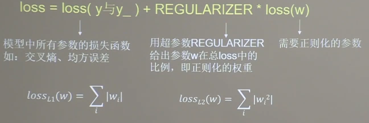
正则化的选择
- L1正则化大概率会使很多参数变为0,因此该方法可以通过稀释参数,即减少参数的数量,降低复杂度。
- L2正则化会使参数很接近但不为0,因此该方法可以通过减小参数值的大小降低复杂度
下面正则化缓解过拟合案例需要使用要以下数据,数据文件名字为dot.csv。该文件应该和代码在同一目录下。
- x1,x2,y_c
- -0.416757847,-0.056266827,1
- -2.136196096,1.640270808,0
- -1.793435585,-0.841747366,0
- 0.502881417,-1.245288087,1
- -1.057952219,-0.909007615,1
- 0.551454045,2.292208013,0
- 0.041539393,-1.117925445,1
- 0.539058321,-0.5961597,1
- -0.019130497,1.17500122,1
- -0.747870949,0.009025251,1
- -0.878107893,-0.15643417,1
- 0.256570452,-0.988779049,1
- -0.338821966,-0.236184031,1
- -0.637655012,-1.187612286,1
- -1.421217227,-0.153495196,0
- -0.26905696,2.231366789,0
- -2.434767577,0.112726505,0
- 0.370444537,1.359633863,1
- 0.501857207,-0.844213704,1
- 9.76E-06,0.542352572,1
- -0.313508197,0.771011738,1
- -1.868090655,1.731184666,0
- 1.467678011,-0.335677339,0
- 0.61134078,0.047970592,1
- -0.829135289,0.087710218,1
- 1.000365887,-0.381092518,1
- -0.375669423,-0.074470763,1
- 0.43349633,1.27837923,1
- -0.634679305,0.508396243,1
- 0.216116006,-1.858612386,0
- -0.419316482,-0.132328898,1
- -0.03957024,0.326003433,1
- -2.040323049,0.046255523,0
- -0.677675577,-1.439439027,0
- 0.52429643,0.735279576,1
- -0.653250268,0.842456282,1
- -0.381516482,0.066489009,1
- -1.098738947,1.584487056,0
- -2.659449456,-0.091452623,0
- 0.695119605,-2.033466546,0
- -0.189469265,-0.077218665,1
- 0.824703005,1.248212921,0
- -0.403892269,-1.384518667,0
- 1.367235424,1.217885633,0
- -0.462005348,0.350888494,1
- 0.381866234,0.566275441,1
- 0.204207979,1.406696242,0
- -1.737959504,1.040823953,0
- 0.38047197,-0.217135269,1
- 1.173531498,-2.343603191,0
- 1.161521491,0.386078048,1
- -1.133133274,0.433092555,1
- -0.304086439,2.585294868,0
- 1.835332723,0.440689872,0
- -0.719253841,-0.583414595,1
- -0.325049628,-0.560234506,1
- -0.902246068,-0.590972275,1
- -0.276179492,-0.516883894,1
- -0.69858995,-0.928891925,1
- 2.550438236,-1.473173248,0
- -1.021414731,0.432395701,1
- -0.32358007,0.423824708,1
- 0.799179995,1.262613663,0
- 0.751964849,-0.993760983,1
- 1.109143281,-1.764917728,0
- -0.114421297,-0.498174194,1
- -1.060799036,0.591666521,1
- -0.183256574,1.019854729,1
- -1.482465478,0.846311892,0
- 0.497940148,0.126504175,1
- -1.418810551,-0.251774118,0
- -1.546674611,-2.082651936,0
- 3.279745401,0.97086132,0
- 1.792592852,-0.429013319,0
- 0.69619798,0.697416272,1
- 0.601515814,0.003659491,1
- -0.228247558,-2.069612263,0
- 0.610144086,0.4234969,1
- 1.117886733,-0.274242089,1
- 1.741812188,-0.447500876,0
- -1.255427218,0.938163671,0
- -0.46834626,-1.254720307,1
- 0.124823646,0.756502143,1
- 0.241439629,0.497425649,1
- 4.108692624,0.821120877,0
- 1.531760316,-1.985845774,0
- 0.365053516,0.774082033,1
- -0.364479092,-0.875979478,1
- 0.396520159,-0.314617436,1
- -0.593755583,1.149500568,1
- 1.335566168,0.302629336,1
- -0.454227855,0.514370717,1
- 0.829458431,0.630621967,1
- -1.45336435,-0.338017777,0
- 0.359133332,0.622220414,1
- 0.960781945,0.758370347,1
- -1.134318483,-0.707420888,1
- -1.221429165,1.804476642,0
- 0.180409807,0.553164274,1
- 1.033029066,-0.329002435,1
- -1.151002944,-0.426522471,1
- -0.148147191,1.501436915,0
- 0.869598198,-1.087090575,1
- 0.664221413,0.734884668,1
- -1.061365744,-0.108516824,1
- -1.850403974,0.330488064,0
- -0.31569321,-1.350002103,1
- -0.698170998,0.239951198,1
- -0.55294944,0.299526813,1
- 0.552663696,-0.840443012,1
- -0.31227067,2.144678089,0
- 0.121105582,-0.846828752,1
- 0.060462449,-1.33858888,1
- 1.132746076,0.370304843,1
- 1.085806404,0.902179395,1
- 0.39029645,0.975509412,1
- 0.191573647,-0.662209012,1
- -1.023514985,-0.448174823,1
- -2.505458132,1.825994457,0
- -1.714067411,-0.076639564,0
- -1.31756727,-2.025593592,0
- -0.082245375,-0.304666585,1
- -0.15972413,0.54894656,1
- -0.618375485,0.378794466,1
- 0.513251444,-0.334844125,1
- -0.283519516,0.538424263,1
- 0.057250947,0.159088487,1
- -2.374402684,0.058519935,0
- 0.376545911,-0.135479764,1
- 0.335908395,1.904375909,0
- 0.085364433,0.665334278,1
- -0.849995503,-0.852341797,1
- -0.479985112,-1.019649099,1
- -0.007601138,-0.933830661,1
- -0.174996844,-1.437143432,0
- -1.652200291,-0.675661789,0
- -1.067067124,-0.652931145,1
- -0.61209475,-0.351262461,1
- 1.045477988,1.369016024,0
- 0.725353259,-0.359474459,1
- 1.49695179,-1.531111108,0
- -2.023363939,0.267972576,0
- -0.002206445,-0.139291883,1
- 0.032565469,-1.640560225,0
- -1.156699171,1.234034681,0
- 1.028184899,-0.721879726,1
- 1.933156966,-1.070796326,0
- -0.571381608,0.292432067,1
- -1.194999895,-0.487930544,1
- -0.173071165,-0.395346401,1
- 0.870840765,0.592806797,1
- -1.099297309,-0.681530644,1
- 0.180066685,-0.066931044,1
- -0.78774954,0.424753672,1
- 0.819885117,-0.631118683,1
- 0.789059649,-1.621673803,0
- -1.610499259,0.499939764,0
- -0.834515207,-0.996959687,1
- -0.263388077,-0.677360492,1
- 0.327067038,-1.455359445,0
- -0.371519124,3.16096597,0
- 0.109951013,-1.913523218,0
- 0.599820429,0.549384465,1
- 1.383781035,0.148349243,1
- -0.653541444,1.408833984,0
- 0.712061227,-1.800716041,0
- 0.747598942,-0.232897001,1
- 1.11064528,-0.373338813,1
- 0.78614607,0.194168696,1
- 0.586204098,-0.020387292,1
- -0.414408598,0.067313412,1
- 0.631798924,0.417592731,1
- 1.615176269,0.425606211,0
- 0.635363758,2.102229267,0
- 0.066126417,0.535558351,1
- -0.603140792,0.041957629,1
- 1.641914637,0.311697707,0
- 1.4511699,-1.06492788,0
- -1.400845455,0.307525527,0
- -1.369638673,2.670337245,0
- 1.248450298,-1.245726553,0
- -0.167168774,-0.57661093,1
- 0.416021749,-0.057847263,1
- 0.931887358,1.468332133,0
- -0.221320943,-1.173155621,1
- 0.562669078,-0.164515057,1
- 1.144855376,-0.152117687,1
- 0.829789046,0.336065952,1
- -0.189044051,-0.449328601,1
- 0.713524448,2.529734874,0
- 0.837615794,-0.131682403,1
- 0.707592866,0.114053878,1
- -1.280895178,0.309846277,1
- 1.548290694,-0.315828043,0
- -1.125903781,0.488496666,1
- 1.830946657,0.940175993,0
- 1.018717047,2.302378289,0
- 1.621092978,0.712683273,0
- -0.208703629,0.137617991,1
- -0.103352168,0.848350567,1
- -0.883125561,1.545386826,0
- 0.145840073,-0.400106056,1
- 0.815206041,-2.074922365,0
- -0.834437391,-0.657718447,1
- 0.820564332,-0.489157001,1
- 1.424967034,-0.446857897,0
- 0.521109431,-0.70819438,1
- 1.15553059,-0.254530459,1
- 0.518924924,-0.492994911,1
- -1.086548153,-0.230917497,1
- 1.098010039,-1.01787805,0
- -1.529391355,-0.307987737,0
- 0.780754356,-1.055839639,1
- -0.543883381,0.184301739,1
- -0.330675843,0.287208202,1
- 1.189528137,0.021201548,1
- -0.06540968,0.766115904,1
- -0.061635085,-0.952897152,1
- -1.014463064,-1.115263963,0
- 1.912600678,-0.045263203,0
- 0.576909718,0.717805695,1
- -0.938998998,0.628775807,1
- -0.564493432,-2.087807462,0
- -0.215050132,-1.075028564,1
- -0.337972149,0.343212732,1
- 2.28253964,-0.495778848,0
- -0.163962832,0.371622161,1
- 0.18652152,-0.158429224,1
- -1.082929557,-0.95662552,0
- -0.183376735,-1.159806896,1
- -0.657768362,-1.251448406,1
- 1.124482861,-1.497839806,0
- 1.902017223,-0.580383038,0
- -1.054915674,-1.182757204,0
- 0.779480054,1.026597951,1
- -0.848666001,0.331539648,1
- -0.149591353,-0.2424406,1
- 0.151197175,0.765069481,1
- -1.916630519,-2.227341292,0
- 0.206689897,-0.070876356,1
- 0.684759969,-1.707539051,0
- -0.986569665,1.543536339,0
- -1.310270529,0.363433972,1
- -0.794872445,-0.405286267,1
- -1.377757931,1.186048676,0
- -1.903821143,-1.198140378,0
- -0.910065643,1.176454193,0
- 0.29921067,0.679267178,1
- -0.01766068,0.236040923,1
- 0.494035871,1.546277646,0
- 0.246857508,-1.468775799,0
- 1.147099942,0.095556985,1
- -1.107438726,-0.176286141,1
- -0.982755667,2.086682727,0
- -0.344623671,-2.002079233,0
- 0.303234433,-0.829874845,1
- 1.288769407,0.134925462,1
- -1.778600641,-0.50079149,0
- -1.088161569,-0.757855553,1
- -0.6437449,-2.008784527,0
- 0.196262894,-0.87589637,1
- -0.893609209,0.751902355,1
- 1.896932244,-0.629079151,0
- 1.812085527,-2.056265741,0
- 0.562704887,-0.582070757,1
- -0.074002975,-0.986496364,1
- -0.594722499,-0.314811843,1
- -0.346940532,0.411443516,1
- 2.326390901,-0.634053128,0
- -0.154409962,-1.749288804,0
- -2.519579296,1.391162427,0
- -1.329346443,-0.745596414,0
- 0.02126085,0.910917515,1
- 0.315276082,1.866208205,0
- -0.182497623,-1.82826634,0
- 0.138955717,0.119450165,1
- -0.8188992,-0.332639265,1
- -0.586387955,1.734516344,0
- -0.612751558,-1.393442017,0
- 0.279433757,-1.822231268,0
- 0.427017458,0.406987749,1
- -0.844308241,-0.559820113,1
- -0.600520405,1.614873237,0
- 0.39495322,-1.203813469,1
- -1.247472432,-0.07754625,1
- -0.013339751,-0.76832325,1
- 0.29123401,-0.197330948,1
- 1.07682965,0.437410232,1
- -0.093197866,0.135631416,1
- -0.882708822,0.884744194,1
- 0.383204463,-0.416994149,1
- 0.11779655,-0.536685309,1
- 2.487184575,-0.451361054,0
- 0.518836127,0.364448005,1
- -0.798348729,0.005657797,1
- -0.320934708,0.24951355,1
- 0.256308392,0.767625083,1
- 0.783020087,-0.407063047,1
- -0.524891667,-0.589808683,1
- -0.862531086,-1.742872904,0
- # 读入数据/标签 生成x_train y_train
- df = pd.read_csv('dot.csv')
- x_data = np.array(df[['x1', 'x2']])
- y_data = np.array(df['y_c'])
-
- x_train = np.vstack(x_data).reshape(-1, 2)
- y_train = np.vstack(y_data).reshape(-1, 1)
-
- Y_c = [['red' if y else 'blue'] for y in y_train]
-
- # 转换x的数据类型,否则后面矩阵相乘时会因数据类型问题报错
- x_train = tf.cast(x_train, tf.float32)
- y_train = tf.cast(y_train, tf.float32)
-
- # from_tensor_slices函数切分传入的张量的第一个维度,生成相应的数据集,使输入特征和标签值一一对应
- train_db = tf.data.Dataset.from_tensor_slices((x_train, y_train)).batch(32) # 打包成数据集
-
- # 生成神经网络的参数,输入层为2个神经元,隐藏层为11个神经元,1层隐藏层,输出层为1个神经元
- # 用tf.Variable()保证参数可训练
- w1 = tf.Variable(tf.random.normal([2, 11]), dtype=tf.float32)
- b1 = tf.Variable(tf.constant(0.01, shape=[11]))
- # 第二层的输入特征个数就是第一层的输出个数,因此11保持一致。为什么是11?随便选的神经元个数,可以更改以改进网络效果
- w2 = tf.Variable(tf.random.normal([11, 1]), dtype=tf.float32)
- b2 = tf.Variable(tf.constant(0.01, shape=[1]))
-
- lr = 0.005 # 学习率
- epoch = 800 # 循环轮数
-
- # 训练部分
- for epoch in range(epoch):
- for step, (x_train, y_train) in enumerate(train_db):
- with tf.GradientTape() as tape: # 记录梯度信息
-
- h1 = tf.matmul(x_train, w1) + b1 # 记录神经网络乘加运算
- h1 = tf.nn.relu(h1)
- y = tf.matmul(h1, w2) + b2
-
- # 采用均方误差损失函数mse = mean(sum(y-out)^2)
- loss = tf.reduce_mean(tf.square(y_train - y))
-
- # 计算loss对各个参数的梯度
- variables = [w1, b1, w2, b2]
- grads = tape.gradient(loss, variables)
-
- # 实现梯度更新
- # w1 = w1 - lr * w1_grad tape.gradient是自动求导结果与[w1, b1, w2, b2] 索引为0,1,2,3
- w1.assign_sub(lr * grads[0])
- b1.assign_sub(lr * grads[1])
- w2.assign_sub(lr * grads[2])
- b2.assign_sub(lr * grads[3])
-
- # 每20个epoch,打印loss信息
- if epoch % 20 == 0:
- print('epoch:', epoch, 'loss:', float(loss))
-
- # 预测部分
- print("*******predict*******")
- # xx在-3到3之间以步长为0.01,yy在-3到3之间以步长0.01,生成间隔数值点
- xx, yy = np.mgrid[-3:3:.1, -3:3:.1]
- # 将xx , yy拉直,并合并配对为二维张量,生成二维坐标点
- grid = np.c_[xx.ravel(), yy.ravel()]
- grid = tf.cast(grid, tf.float32)
- # 将网格坐标点喂入神经网络,进行预测,probs为输出
- probs = []
- for x_test in grid:
- # 使用训练好的参数进行预测
- h1 = tf.matmul([x_test], w1) + b1
- h1 = tf.nn.relu(h1)
- y = tf.matmul(h1, w2) + b2 # y为预测结果
- probs.append(y)
-
- # 取第0列给x1,取第1列给x2
- x1 = x_data[:, 0]
- x2 = x_data[:, 1]
- # probs的shape调整成xx的样子
- probs = np.array(probs).reshape(xx.shape)
- plt.scatter(x1, x2, color=np.squeeze(Y_c)) # squeeze去掉纬度是1的纬度,相当于去掉[['red'],[''blue]],内层括号变为['red','blue']
- # 把坐标xx yy和对应的值probs放入contour函数,给probs值为0.5的所有点上色 plt.show()后 显示的是红蓝点的分界线
- plt.contour(xx, yy, probs, levels=[.5])
- plt.show()
-
- # 读入红蓝点,画出分割线,不包含正则化
- # 不清楚的数据,建议print出来查看
- epoch: 0 loss: 3.3588955402374268
- epoch: 20 loss: 0.0404302217066288
- epoch: 40 loss: 0.04070901498198509
- epoch: 60 loss: 0.03821190819144249
- epoch: 80 loss: 0.036114610731601715
- epoch: 100 loss: 0.03467976301908493
- epoch: 120 loss: 0.03373105823993683
- epoch: 140 loss: 0.03225767984986305
- epoch: 160 loss: 0.03019583784043789
- epoch: 180 loss: 0.028336063027381897
- epoch: 200 loss: 0.026807844638824463
- epoch: 220 loss: 0.025512710213661194
- epoch: 240 loss: 0.024442538619041443
- epoch: 260 loss: 0.02359318919479847
- epoch: 280 loss: 0.022960280999541283
- epoch: 300 loss: 0.02251446805894375
- epoch: 320 loss: 0.02214951254427433
- epoch: 340 loss: 0.02189861238002777
- epoch: 360 loss: 0.021764680743217468
- epoch: 380 loss: 0.021699346601963043
- epoch: 400 loss: 0.021605348214507103
- epoch: 420 loss: 0.021516701206564903
- epoch: 440 loss: 0.021409569308161736
- epoch: 460 loss: 0.02125600166618824
- epoch: 480 loss: 0.021161897107958794
- epoch: 500 loss: 0.021076681092381477
- epoch: 520 loss: 0.02100759744644165
- epoch: 540 loss: 0.020953044295310974
- epoch: 560 loss: 0.020902445539832115
- epoch: 580 loss: 0.020858166739344597
- epoch: 600 loss: 0.02082127146422863
- epoch: 620 loss: 0.020805032923817635
- epoch: 640 loss: 0.020836150273680687
- epoch: 660 loss: 0.020815739408135414
- epoch: 680 loss: 0.02078959532082081
- epoch: 700 loss: 0.020798802375793457
- epoch: 720 loss: 0.020799407735466957
- epoch: 740 loss: 0.020800543949007988
- epoch: 760 loss: 0.020800618454813957
- epoch: 780 loss: 0.020786955952644348
- *******predict*******

神经网络参数优化器
待优化参数w;损失函数loss;学习率lr;每次迭代一个vatch;t表示当前batch总次数
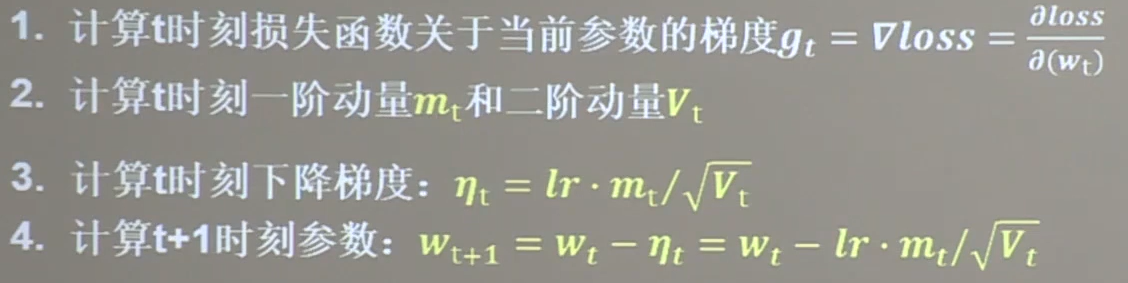
一阶动量:与梯度相关的函数
二阶动量:与梯度平方相关的函数
优化器
SGD

无momentum:不含动量
mt=gt 一阶动量定义为梯度
Vt= 1 二阶动量恒等于1
ηt = 学习率lr 乘以 一阶动量 除以 二阶动量开平方 = lr * gt
最后方框框起来的是需要记住的参数更新公式
对于单层网络:
- w1.assign_sub(lr * grads[0]) # 参数w1自更新
- b1.assign_sub(lr * grads[1]) # 参数b自更新
- from sklearn import datasets
- import time ##1##
-
- # 导入数据,分别为输入特征和标签
- x_data = datasets.load_iris().data
- y_data = datasets.load_iris().target
-
- # 随机打乱数据(因为原始数据是顺序的,顺序不打乱会影响准确率)
- # seed: 随机数种子,是一个整数,当设置之后,每次生成的随机数都一样(为方便教学,以保每位同学结果一致)
- np.random.seed(116) # 使用相同的seed,保证输入特征和标签一一对应
- np.random.shuffle(x_data)
- np.random.seed(116)
- np.random.shuffle(y_data)
- tf.random.set_seed(116)
-
- # 将打乱后的数据集分割为训练集和测试集,训练集为前120行,测试集为后30行
- x_train = x_data[:-30]
- y_train = y_data[:-30]
- x_test = x_data[-30:]
- y_test = y_data[-30:]
-
- # 转换x的数据类型,否则后面矩阵相乘时会因数据类型不一致报错
- x_train = tf.cast(x_train, tf.float32)
- x_test = tf.cast(x_test, tf.float32)
-
- # from_tensor_slices函数使输入特征和标签值一一对应。(把数据集分批次,每个批次batch组数据)
- train_db = tf.data.Dataset.from_tensor_slices((x_train, y_train)).batch(32)
- test_db = tf.data.Dataset.from_tensor_slices((x_test, y_test)).batch(32)
-
- # 生成神经网络的参数,4个输入特征故,输入层为4个输入节点;因为3分类,故输出层为3个神经元
- # 用tf.Variable()标记参数可训练
- # 使用seed使每次生成的随机数相同(方便教学,使大家结果都一致,在现实使用时不写seed)
- w1 = tf.Variable(tf.random.truncated_normal([4, 3], stddev=0.1, seed=1))
- b1 = tf.Variable(tf.random.truncated_normal([3], stddev=0.1, seed=1))
-
- lr = 0.1 # 学习率为0.1
- train_loss_results = [] # 将每轮的loss记录在此列表中,为后续画loss曲线提供数据
- test_acc = [] # 将每轮的acc记录在此列表中,为后续画acc曲线提供数据
- epoch = 500 # 循环500轮
- loss_all = 0 # 每轮分4个step,loss_all记录四个step生成的4个loss的和
-
- # 训练部分
- now_time = time.time() ##2##
- for epoch in range(epoch): # 数据集级别的循环,每个epoch循环一次数据集
- for step, (x_train, y_train) in enumerate(train_db): # batch级别的循环 ,每个step循环一个batch
- with tf.GradientTape() as tape: # with结构记录梯度信息
- y = tf.matmul(x_train, w1) + b1 # 神经网络乘加运算
- y = tf.nn.softmax(y) # 使输出y符合概率分布(此操作后与独热码同量级,可相减求loss)
- y_ = tf.one_hot(y_train, depth=3) # 将标签值转换为独热码格式,方便计算loss和accuracy
- loss = tf.reduce_mean(tf.square(y_ - y)) # 采用均方误差损失函数mse = mean(sum(y-out)^2)
- loss_all += loss.numpy() # 将每个step计算出的loss累加,为后续求loss平均值提供数据,这样计算的loss更准确
- # 计算loss对各个参数的梯度
- grads = tape.gradient(loss, [w1, b1])
-
- # 实现梯度更新 w1 = w1 - lr * w1_grad b = b - lr * b_grad
- w1.assign_sub(lr * grads[0]) # 参数w1自更新
- b1.assign_sub(lr * grads[1]) # 参数b自更新
-
- # 每个epoch,打印loss信息
- # print("Epoch {}, loss: {}".format(epoch, loss_all / 4))
- train_loss_results.append(loss_all / 4) # 将4个step的loss求平均记录在此变量中
- loss_all = 0 # loss_all归零,为记录下一个epoch的loss做准备
-
- # 测试部分
- # total_correct为预测对的样本个数, total_number为测试的总样本数,将这两个变量都初始化为0
- total_correct, total_number = 0, 0
- for x_test, y_test in test_db:
- # 使用更新后的参数进行预测
- y = tf.matmul(x_test, w1) + b1
- y = tf.nn.softmax(y)
- pred = tf.argmax(y, axis=1) # 返回y中最大值的索引,即预测的分类
- # 将pred转换为y_test的数据类型
- pred = tf.cast(pred, dtype=y_test.dtype)
- # 若分类正确,则correct=1,否则为0,将bool型的结果转换为int型
- correct = tf.cast(tf.equal(pred, y_test), dtype=tf.int32)
- # 将每个batch的correct数加起来
- correct = tf.reduce_sum(correct)
- # 将所有batch中的correct数加起来
- total_correct += int(correct)
- # total_number为测试的总样本数,也就是x_test的行数,shape[0]返回变量的行数
- total_number += x_test.shape[0]
- # 总的准确率等于total_correct/total_number
- acc = total_correct / total_number
- test_acc.append(acc)
- # print("Test_acc:", acc)
- # print("--------------------------")
- total_time = time.time() - now_time ##3##
- print("total_time", total_time) ##4##
-
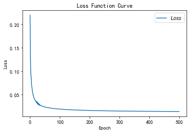
- # 绘制 loss 曲线
- plt.title('Loss Function Curve') # 图片标题
- plt.xlabel('Epoch') # x轴变量名称
- plt.ylabel('Loss') # y轴变量名称
- plt.plot(train_loss_results, label="$Loss$") # 逐点画出trian_loss_results值并连线,连线图标是Loss
- plt.legend() # 画出曲线图标
- plt.show() # 画出图像
-
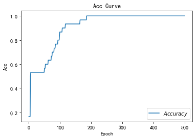
- # 绘制 Accuracy 曲线
- plt.title('Acc Curve') # 图片标题
- plt.xlabel('Epoch') # x轴变量名称
- plt.ylabel('Acc') # y轴变量名称
- plt.plot(test_acc, label="$Accuracy$") # 逐点画出test_acc值并连线,连线图标是Accuracy
- plt.legend()
- plt.show()
-
- # 本文件较 class1\p45_iris.py 仅添加四处时间记录 用 ##n## 标识
- # 请将loss曲线、ACC曲线、total_time记录到 class2\优化器对比.docx 对比各优化器收敛情况
total_time 3.9469685554504395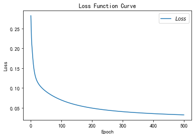
SGDM

mt这个公式表示各时刻梯度方向的指数滑动平均值
mt-1表示上一时刻的一阶动量
β是个超参数,是个接近1的数值,因此β* mt-1 在公式中占大头
- m_w,m_b = 0,0 # 第一个时刻的一阶动量是由第0时刻的一阶动量决定,而第0时刻的一阶动量为0
- beta = 0.9
-
- # sgd-momentun
-
- m_w = beta * m_w + (1 - beta) * grads[0]
- m_b = beta * m_b + (1 - beta) * grads[1]
-
- w1.assign_sub(lr * m_w)
- b1.assign_sub(lr * m_b)
- # 导入数据,分别为输入特征和标签
- x_data = datasets.load_iris().data
- y_data = datasets.load_iris().target
-
- # 随机打乱数据(因为原始数据是顺序的,顺序不打乱会影响准确率)
- # seed: 随机数种子,是一个整数,当设置之后,每次生成的随机数都一样(为方便教学,以保每位同学结果一致)
- np.random.seed(116) # 使用相同的seed,保证输入特征和标签一一对应
- np.random.shuffle(x_data)
- np.random.seed(116)
- np.random.shuffle(y_data)
- tf.random.set_seed(116)
-
- # 将打乱后的数据集分割为训练集和测试集,训练集为前120行,测试集为后30行
- x_train = x_data[:-30]
- y_train = y_data[:-30]
- x_test = x_data[-30:]
- y_test = y_data[-30:]
-
- # 转换x的数据类型,否则后面矩阵相乘时会因数据类型不一致报错
- x_train = tf.cast(x_train, tf.float32)
- x_test = tf.cast(x_test, tf.float32)
-
- # from_tensor_slices函数使输入特征和标签值一一对应。(把数据集分批次,每个批次batch组数据)
- train_db = tf.data.Dataset.from_tensor_slices((x_train, y_train)).batch(32)
- test_db = tf.data.Dataset.from_tensor_slices((x_test, y_test)).batch(32)
-
- # 生成神经网络的参数,4个输入特征故,输入层为4个输入节点;因为3分类,故输出层为3个神经元
- # 用tf.Variable()标记参数可训练
- # 使用seed使每次生成的随机数相同(方便教学,使大家结果都一致,在现实使用时不写seed)
- w1 = tf.Variable(tf.random.truncated_normal([4, 3], stddev=0.1, seed=1))
- b1 = tf.Variable(tf.random.truncated_normal([3], stddev=0.1, seed=1))
-
- lr = 0.1 # 学习率为0.1
- train_loss_results = [] # 将每轮的loss记录在此列表中,为后续画loss曲线提供数据
- test_acc = [] # 将每轮的acc记录在此列表中,为后续画acc曲线提供数据
- epoch = 500 # 循环500轮
- loss_all = 0 # 每轮分4个step,loss_all记录四个step生成的4个loss的和
-
- ##########################################################################
- m_w, m_b = 0, 0
- beta = 0.9
- ##########################################################################
-
- # 训练部分
- now_time = time.time() ##2##
- for epoch in range(epoch): # 数据集级别的循环,每个epoch循环一次数据集
- for step, (x_train, y_train) in enumerate(train_db): # batch级别的循环 ,每个step循环一个batch
- with tf.GradientTape() as tape: # with结构记录梯度信息
- y = tf.matmul(x_train, w1) + b1 # 神经网络乘加运算
- y = tf.nn.softmax(y) # 使输出y符合概率分布(此操作后与独热码同量级,可相减求loss)
- y_ = tf.one_hot(y_train, depth=3) # 将标签值转换为独热码格式,方便计算loss和accuracy
- loss = tf.reduce_mean(tf.square(y_ - y)) # 采用均方误差损失函数mse = mean(sum(y-out)^2)
- loss_all += loss.numpy() # 将每个step计算出的loss累加,为后续求loss平均值提供数据,这样计算的loss更准确
- # 计算loss对各个参数的梯度
- grads = tape.gradient(loss, [w1, b1])
-
- ##########################################################################
- # sgd-momentun
- m_w = beta * m_w + (1 - beta) * grads[0]
- m_b = beta * m_b + (1 - beta) * grads[1]
- w1.assign_sub(lr * m_w)
- b1.assign_sub(lr * m_b)
- ##########################################################################
-
- # 每个epoch,打印loss信息
- # print("Epoch {}, loss: {}".format(epoch, loss_all / 4))
- train_loss_results.append(loss_all / 4) # 将4个step的loss求平均记录在此变量中
- loss_all = 0 # loss_all归零,为记录下一个epoch的loss做准备
-
- # 测试部分
- # total_correct为预测对的样本个数, total_number为测试的总样本数,将这两个变量都初始化为0
- total_correct, total_number = 0, 0
- for x_test, y_test in test_db:
- # 使用更新后的参数进行预测
- y = tf.matmul(x_test, w1) + b1
- y = tf.nn.softmax(y)
- pred = tf.argmax(y, axis=1) # 返回y中最大值的索引,即预测的分类
- # 将pred转换为y_test的数据类型
- pred = tf.cast(pred, dtype=y_test.dtype)
- # 若分类正确,则correct=1,否则为0,将bool型的结果转换为int型
- correct = tf.cast(tf.equal(pred, y_test), dtype=tf.int32)
- # 将每个batch的correct数加起来
- correct = tf.reduce_sum(correct)
- # 将所有batch中的correct数加起来
- total_correct += int(correct)
- # total_number为测试的总样本数,也就是x_test的行数,shape[0]返回变量的行数
- total_number += x_test.shape[0]
- # 总的准确率等于total_correct/total_number
- acc = total_correct / total_number
- test_acc.append(acc)
- # print("Test_acc:", acc)
- # print("--------------------------")
- total_time = time.time() - now_time ##3##
- print("total_time", total_time) ##4##
-
- # 绘制 loss 曲线
- plt.title('Loss Function Curve') # 图片标题
- plt.xlabel('Epoch') # x轴变量名称
- plt.ylabel('Loss') # y轴变量名称
- plt.plot(train_loss_results, label="$Loss$") # 逐点画出trian_loss_results值并连线,连线图标是Loss
- plt.legend() # 画出曲线图标
- plt.show() # 画出图像
-
- # 绘制 Accuracy 曲线
- plt.title('Acc Curve') # 图片标题
- plt.xlabel('Epoch') # x轴变量名称
- plt.ylabel('Acc') # y轴变量名称
- plt.plot(test_acc, label="$Accuracy$") # 逐点画出test_acc值并连线,连线图标是Accuracy
- plt.legend()
- plt.show()
-
- # 请将loss曲线、ACC曲线、total_time记录到 class2\优化器对比.docx 对比各优化器收敛情况
total_time 4.3680760860443115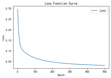

Adagrad

- v_w += tf.square(grads[0])
- v_b += tf.square(grads[1])
- w1.assign_sub(lr * grads[0] / tf.sqrt(v_w))
- b1.assign_sub(lr * grads[1] / tf.sqrt(v_b))
- # 导入数据,分别为输入特征和标签
- x_data = datasets.load_iris().data
- y_data = datasets.load_iris().target
-
- # 随机打乱数据(因为原始数据是顺序的,顺序不打乱会影响准确率)
- # seed: 随机数种子,是一个整数,当设置之后,每次生成的随机数都一样(为方便教学,以保每位同学结果一致)
- np.random.seed(116) # 使用相同的seed,保证输入特征和标签一一对应
- np.random.shuffle(x_data)
- np.random.seed(116)
- np.random.shuffle(y_data)
- tf.random.set_seed(116)
-
- # 将打乱后的数据集分割为训练集和测试集,训练集为前120行,测试集为后30行
- x_train = x_data[:-30]
- y_train = y_data[:-30]
- x_test = x_data[-30:]
- y_test = y_data[-30:]
-
- # 转换x的数据类型,否则后面矩阵相乘时会因数据类型不一致报错
- x_train = tf.cast(x_train, tf.float32)
- x_test = tf.cast(x_test, tf.float32)
-
- # from_tensor_slices函数使输入特征和标签值一一对应。(把数据集分批次,每个批次batch组数据)
- train_db = tf.data.Dataset.from_tensor_slices((x_train, y_train)).batch(32)
- test_db = tf.data.Dataset.from_tensor_slices((x_test, y_test)).batch(32)
-
- # 生成神经网络的参数,4个输入特征故,输入层为4个输入节点;因为3分类,故输出层为3个神经元
- # 用tf.Variable()标记参数可训练
- # 使用seed使每次生成的随机数相同(方便教学,使大家结果都一致,在现实使用时不写seed)
- w1 = tf.Variable(tf.random.truncated_normal([4, 3], stddev=0.1, seed=1))
- b1 = tf.Variable(tf.random.truncated_normal([3], stddev=0.1, seed=1))
-
- lr = 0.1 # 学习率为0.1
- train_loss_results = [] # 将每轮的loss记录在此列表中,为后续画loss曲线提供数据
- test_acc = [] # 将每轮的acc记录在此列表中,为后续画acc曲线提供数据
- epoch = 500 # 循环500轮
- loss_all = 0 # 每轮分4个step,loss_all记录四个step生成的4个loss的和
-
- ##########################################################################
- v_w, v_b = 0, 0
- ##########################################################################
-
- # 训练部分
- now_time = time.time() ##2##
- for epoch in range(epoch): # 数据集级别的循环,每个epoch循环一次数据集
- for step, (x_train, y_train) in enumerate(train_db): # batch级别的循环 ,每个step循环一个batch
- with tf.GradientTape() as tape: # with结构记录梯度信息
- y = tf.matmul(x_train, w1) + b1 # 神经网络乘加运算
- y = tf.nn.softmax(y) # 使输出y符合概率分布(此操作后与独热码同量级,可相减求loss)
- y_ = tf.one_hot(y_train, depth=3) # 将标签值转换为独热码格式,方便计算loss和accuracy
- loss = tf.reduce_mean(tf.square(y_ - y)) # 采用均方误差损失函数mse = mean(sum(y-out)^2)
- loss_all += loss.numpy() # 将每个step计算出的loss累加,为后续求loss平均值提供数据,这样计算的loss更准确
- # 计算loss对各个参数的梯度
- grads = tape.gradient(loss, [w1, b1])
-
- ##########################################################################
- # adagrad
- v_w += tf.square(grads[0])
- v_b += tf.square(grads[1])
- w1.assign_sub(lr * grads[0] / tf.sqrt(v_w))
- b1.assign_sub(lr * grads[1] / tf.sqrt(v_b))
- ##########################################################################
-
- # 每个epoch,打印loss信息
- # print("Epoch {}, loss: {}".format(epoch, loss_all / 4))
- train_loss_results.append(loss_all / 4) # 将4个step的loss求平均记录在此变量中
- loss_all = 0 # loss_all归零,为记录下一个epoch的loss做准备
-
- # 测试部分
- # total_correct为预测对的样本个数, total_number为测试的总样本数,将这两个变量都初始化为0
- total_correct, total_number = 0, 0
- for x_test, y_test in test_db:
- # 使用更新后的参数进行预测
- y = tf.matmul(x_test, w1) + b1
- y = tf.nn.softmax(y)
- pred = tf.argmax(y, axis=1) # 返回y中最大值的索引,即预测的分类
- # 将pred转换为y_test的数据类型
- pred = tf.cast(pred, dtype=y_test.dtype)
- # 若分类正确,则correct=1,否则为0,将bool型的结果转换为int型
- correct = tf.cast(tf.equal(pred, y_test), dtype=tf.int32)
- # 将每个batch的correct数加起来
- correct = tf.reduce_sum(correct)
- # 将所有batch中的correct数加起来
- total_correct += int(correct)
- # total_number为测试的总样本数,也就是x_test的行数,shape[0]返回变量的行数
- total_number += x_test.shape[0]
- # 总的准确率等于total_correct/total_number
- acc = total_correct / total_number
- test_acc.append(acc)
- # print("Test_acc:", acc)
- # print("--------------------------")
- total_time = time.time() - now_time ##3##
- print("total_time", total_time) ##4##
-
- # 绘制 loss 曲线
- plt.title('Loss Function Curve') # 图片标题
- plt.xlabel('Epoch') # x轴变量名称
- plt.ylabel('Loss') # y轴变量名称
- plt.plot(train_loss_results, label="$Loss$") # 逐点画出trian_loss_results值并连线,连线图标是Loss
- plt.legend() # 画出曲线图标
- plt.show() # 画出图像
-
- # 绘制 Accuracy 曲线
- plt.title('Acc Curve') # 图片标题
- plt.xlabel('Epoch') # x轴变量名称
- plt.ylabel('Acc') # y轴变量名称
- plt.plot(test_acc, label="$Accuracy$") # 逐点画出test_acc值并连线,连线图标是Accuracy
- plt.legend()
- plt.show()
-
- # 请将loss曲线、ACC曲线、total_time记录到 class2\优化器对比.docx 对比各优化器收敛情况
total_time 4.468905210494995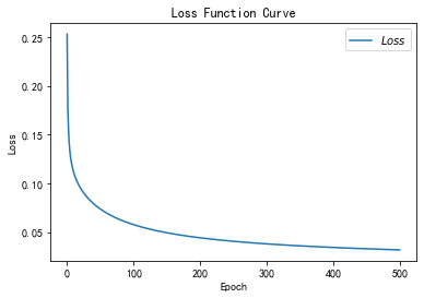

RMSProp

二阶动量v使用指数滑动平均值计算,表征的是过去一段时间的平均值
表征,是信息在头脑中的呈现方式,是信息记载或表达的方式,能把某些实体或某类信息表达清楚的形式化系统以及说明该系统如何行使其职能的若干规则。因此,我们可以这样理解,表征是指可以指代某种东西的符号或信号,即某一事物缺席时,它代表该事物。@百度百科-表征
- v_w ,v_b = 0,0
- beta = 0.9
-
- v_w = beta * v_w + (1 - beta) * tf.square(grads[0])
- v_b = beta * v_b + (1 - beta) * tf.square(grads[1])
- w1.assign_sub(lr * grads[0] / tf.sqrt(v_w))
- b1.assign_sub(lr * grads[1] / tf.sqrt(v_b))
- # 导入数据,分别为输入特征和标签
- x_data = datasets.load_iris().data
- y_data = datasets.load_iris().target
-
- # 随机打乱数据(因为原始数据是顺序的,顺序不打乱会影响准确率)
- # seed: 随机数种子,是一个整数,当设置之后,每次生成的随机数都一样(为方便教学,以保每位同学结果一致)
- np.random.seed(116) # 使用相同的seed,保证输入特征和标签一一对应
- np.random.shuffle(x_data)
- np.random.seed(116)
- np.random.shuffle(y_data)
- tf.random.set_seed(116)
-
- # 将打乱后的数据集分割为训练集和测试集,训练集为前120行,测试集为后30行
- x_train = x_data[:-30]
- y_train = y_data[:-30]
- x_test = x_data[-30:]
- y_test = y_data[-30:]
-
- # 转换x的数据类型,否则后面矩阵相乘时会因数据类型不一致报错
- x_train = tf.cast(x_train, tf.float32)
- x_test = tf.cast(x_test, tf.float32)
-
- # from_tensor_slices函数使输入特征和标签值一一对应。(把数据集分批次,每个批次batch组数据)
- train_db = tf.data.Dataset.from_tensor_slices((x_train, y_train)).batch(32)
- test_db = tf.data.Dataset.from_tensor_slices((x_test, y_test)).batch(32)
-
- # 生成神经网络的参数,4个输入特征故,输入层为4个输入节点;因为3分类,故输出层为3个神经元
- # 用tf.Variable()标记参数可训练
- # 使用seed使每次生成的随机数相同(方便教学,使大家结果都一致,在现实使用时不写seed)
- w1 = tf.Variable(tf.random.truncated_normal([4, 3], stddev=0.1, seed=1))
- b1 = tf.Variable(tf.random.truncated_normal([3], stddev=0.1, seed=1))
-
- lr = 0.1 # 学习率为0.1
- train_loss_results = [] # 将每轮的loss记录在此列表中,为后续画loss曲线提供数据
- test_acc = [] # 将每轮的acc记录在此列表中,为后续画acc曲线提供数据
- epoch = 500 # 循环500轮
- loss_all = 0 # 每轮分4个step,loss_all记录四个step生成的4个loss的和
-
- ##########################################################################
- v_w, v_b = 0, 0
- beta = 0.9
- ##########################################################################
-
- # 训练部分
- now_time = time.time() ##2##
- for epoch in range(epoch): # 数据集级别的循环,每个epoch循环一次数据集
- for step, (x_train, y_train) in enumerate(train_db): # batch级别的循环 ,每个step循环一个batch
- with tf.GradientTape() as tape: # with结构记录梯度信息
- y = tf.matmul(x_train, w1) + b1 # 神经网络乘加运算
- y = tf.nn.softmax(y) # 使输出y符合概率分布(此操作后与独热码同量级,可相减求loss)
- y_ = tf.one_hot(y_train, depth=3) # 将标签值转换为独热码格式,方便计算loss和accuracy
- loss = tf.reduce_mean(tf.square(y_ - y)) # 采用均方误差损失函数mse = mean(sum(y-out)^2)
- loss_all += loss.numpy() # 将每个step计算出的loss累加,为后续求loss平均值提供数据,这样计算的loss更准确
- # 计算loss对各个参数的梯度
- grads = tape.gradient(loss, [w1, b1])
-
- ##########################################################################
- # rmsprop
- v_w = beta * v_w + (1 - beta) * tf.square(grads[0])
- v_b = beta * v_b + (1 - beta) * tf.square(grads[1])
- w1.assign_sub(lr * grads[0] / tf.sqrt(v_w))
- b1.assign_sub(lr * grads[1] / tf.sqrt(v_b))
- ##########################################################################
-
- # 每个epoch,打印loss信息
- # print("Epoch {}, loss: {}".format(epoch, loss_all / 4))
- train_loss_results.append(loss_all / 4) # 将4个step的loss求平均记录在此变量中
- loss_all = 0 # loss_all归零,为记录下一个epoch的loss做准备
-
- # 测试部分
- # total_correct为预测对的样本个数, total_number为测试的总样本数,将这两个变量都初始化为0
- total_correct, total_number = 0, 0
- for x_test, y_test in test_db:
- # 使用更新后的参数进行预测
- y = tf.matmul(x_test, w1) + b1
- y = tf.nn.softmax(y)
- pred = tf.argmax(y, axis=1) # 返回y中最大值的索引,即预测的分类
- # 将pred转换为y_test的数据类型
- pred = tf.cast(pred, dtype=y_test.dtype)
- # 若分类正确,则correct=1,否则为0,将bool型的结果转换为int型
- correct = tf.cast(tf.equal(pred, y_test), dtype=tf.int32)
- # 将每个batch的correct数加起来
- correct = tf.reduce_sum(correct)
- # 将所有batch中的correct数加起来
- total_correct += int(correct)
- # total_number为测试的总样本数,也就是x_test的行数,shape[0]返回变量的行数
- total_number += x_test.shape[0]
- # 总的准确率等于total_correct/total_number
- acc = total_correct / total_number
- test_acc.append(acc)
- # print("Test_acc:", acc)
- # print("--------------------------")
- total_time = time.time() - now_time ##3##
- print("total_time", total_time) ##4##
-
- # 绘制 loss 曲线
- plt.title('Loss Function Curve') # 图片标题
- plt.xlabel('Epoch') # x轴变量名称
- plt.ylabel('Loss') # y轴变量名称
- plt.plot(train_loss_results, label="$Loss$") # 逐点画出trian_loss_results值并连线,连线图标是Loss
- plt.legend() # 画出曲线图标
- plt.show() # 画出图像
-
- # 绘制 Accuracy 曲线
- plt.title('Acc Curve') # 图片标题
- plt.xlabel('Epoch') # x轴变量名称
- plt.ylabel('Acc') # y轴变量名称
- plt.plot(test_acc, label="$Accuracy$") # 逐点画出test_acc值并连线,连线图标是Accuracy
- plt.legend()
- plt.show()
-
- # 请将loss曲线、ACC曲线、total_time记录到 class2\优化器对比.docx 对比各优化器收敛情况
total_time 4.61161208152771

Adam

- m_w, m_b = 0, 0
- v_w, v_b = 0, 0
- beta1, beta2 = 0.9, 0.999
- delta_w, delta_b = 0, 0
- global_step = 0
-
- m_w = beta1 * m_w + (1 - beta1) * grads[0]
- m_b = beta1 * m_b + (1 - beta1) * grads[1]
- v_w = beta2 * v_w + (1 - beta2) * tf.square(grads[0])
- v_b = beta2 * v_b + (1 - beta2) * tf.square(grads[1])
-
- m_w_correction = m_w / (1 - tf.pow(beta1, int(global_step)))
- m_b_correction = m_b / (1 - tf.pow(beta1, int(global_step)))
- v_w_correction = v_w / (1 - tf.pow(beta2, int(global_step)))
- v_b_correction = v_b / (1 - tf.pow(beta2, int(global_step)))
-
- w1.assign_sub(lr * m_w_correction / tf.sqrt(v_w_correction))
- b1.assign_sub(lr * m_b_correction / tf.sqrt(v_b_correction))
- # 导入数据,分别为输入特征和标签
- x_data = datasets.load_iris().data
- y_data = datasets.load_iris().target
-
- # 随机打乱数据(因为原始数据是顺序的,顺序不打乱会影响准确率)
- # seed: 随机数种子,是一个整数,当设置之后,每次生成的随机数都一样(为方便教学,以保每位同学结果一致)
- np.random.seed(116) # 使用相同的seed,保证输入特征和标签一一对应
- np.random.shuffle(x_data)
- np.random.seed(116)
- np.random.shuffle(y_data)
- tf.random.set_seed(116)
-
- # 将打乱后的数据集分割为训练集和测试集,训练集为前120行,测试集为后30行
- x_train = x_data[:-30]
- y_train = y_data[:-30]
- x_test = x_data[-30:]
- y_test = y_data[-30:]
-
- # 转换x的数据类型,否则后面矩阵相乘时会因数据类型不一致报错
- x_train = tf.cast(x_train, tf.float32)
- x_test = tf.cast(x_test, tf.float32)
-
- # from_tensor_slices函数使输入特征和标签值一一对应。(把数据集分批次,每个批次batch组数据)
- train_db = tf.data.Dataset.from_tensor_slices((x_train, y_train)).batch(32)
- test_db = tf.data.Dataset.from_tensor_slices((x_test, y_test)).batch(32)
-
- # 生成神经网络的参数,4个输入特征故,输入层为4个输入节点;因为3分类,故输出层为3个神经元
- # 用tf.Variable()标记参数可训练
- # 使用seed使每次生成的随机数相同(方便教学,使大家结果都一致,在现实使用时不写seed)
- w1 = tf.Variable(tf.random.truncated_normal([4, 3], stddev=0.1, seed=1))
- b1 = tf.Variable(tf.random.truncated_normal([3], stddev=0.1, seed=1))
-
- lr = 0.1 # 学习率为0.1
- train_loss_results = [] # 将每轮的loss记录在此列表中,为后续画loss曲线提供数据
- test_acc = [] # 将每轮的acc记录在此列表中,为后续画acc曲线提供数据
- epoch = 500 # 循环500轮
- loss_all = 0 # 每轮分4个step,loss_all记录四个step生成的4个loss的和
-
- ##########################################################################
- m_w, m_b = 0, 0
- v_w, v_b = 0, 0
- beta1, beta2 = 0.9, 0.999
- delta_w, delta_b = 0, 0
- global_step = 0
- ##########################################################################
-
- # 训练部分
- now_time = time.time() ##2##
- for epoch in range(epoch): # 数据集级别的循环,每个epoch循环一次数据集
- for step, (x_train, y_train) in enumerate(train_db): # batch级别的循环 ,每个step循环一个batch
- ##########################################################################
- global_step += 1
- ##########################################################################
- with tf.GradientTape() as tape: # with结构记录梯度信息
- y = tf.matmul(x_train, w1) + b1 # 神经网络乘加运算
- y = tf.nn.softmax(y) # 使输出y符合概率分布(此操作后与独热码同量级,可相减求loss)
- y_ = tf.one_hot(y_train, depth=3) # 将标签值转换为独热码格式,方便计算loss和accuracy
- loss = tf.reduce_mean(tf.square(y_ - y)) # 采用均方误差损失函数mse = mean(sum(y-out)^2)
- loss_all += loss.numpy() # 将每个step计算出的loss累加,为后续求loss平均值提供数据,这样计算的loss更准确
- # 计算loss对各个参数的梯度
- grads = tape.gradient(loss, [w1, b1])
-
- ##########################################################################
- # adam
- m_w = beta1 * m_w + (1 - beta1) * grads[0]
- m_b = beta1 * m_b + (1 - beta1) * grads[1]
- v_w = beta2 * v_w + (1 - beta2) * tf.square(grads[0])
- v_b = beta2 * v_b + (1 - beta2) * tf.square(grads[1])
-
- m_w_correction = m_w / (1 - tf.pow(beta1, int(global_step)))
- m_b_correction = m_b / (1 - tf.pow(beta1, int(global_step)))
- v_w_correction = v_w / (1 - tf.pow(beta2, int(global_step)))
- v_b_correction = v_b / (1 - tf.pow(beta2, int(global_step)))
-
- w1.assign_sub(lr * m_w_correction / tf.sqrt(v_w_correction))
- b1.assign_sub(lr * m_b_correction / tf.sqrt(v_b_correction))
- ##########################################################################
-
- # 每个epoch,打印loss信息
- # print("Epoch {}, loss: {}".format(epoch, loss_all / 4))
- train_loss_results.append(loss_all / 4) # 将4个step的loss求平均记录在此变量中
- loss_all = 0 # loss_all归零,为记录下一个epoch的loss做准备
-
- # 测试部分
- # total_correct为预测对的样本个数, total_number为测试的总样本数,将这两个变量都初始化为0
- total_correct, total_number = 0, 0
- for x_test, y_test in test_db:
- # 使用更新后的参数进行预测
- y = tf.matmul(x_test, w1) + b1
- y = tf.nn.softmax(y)
- pred = tf.argmax(y, axis=1) # 返回y中最大值的索引,即预测的分类
- # 将pred转换为y_test的数据类型
- pred = tf.cast(pred, dtype=y_test.dtype)
- # 若分类正确,则correct=1,否则为0,将bool型的结果转换为int型
- correct = tf.cast(tf.equal(pred, y_test), dtype=tf.int32)
- # 将每个batch的correct数加起来
- correct = tf.reduce_sum(correct)
- # 将所有batch中的correct数加起来
- total_correct += int(correct)
- # total_number为测试的总样本数,也就是x_test的行数,shape[0]返回变量的行数
- total_number += x_test.shape[0]
- # 总的准确率等于total_correct/total_number
- acc = total_correct / total_number
- test_acc.append(acc)
- # print("Test_acc:", acc)
- # print("--------------------------")
- total_time = time.time() - now_time ##3##
- print("total_time", total_time) ##4##
-
- # 绘制 loss 曲线
- plt.title('Loss Function Curve') # 图片标题
- plt.xlabel('Epoch') # x轴变量名称
- plt.ylabel('Loss') # y轴变量名称
- plt.plot(train_loss_results, label="$Loss$") # 逐点画出trian_loss_results值并连线,连线图标是Loss
- plt.legend() # 画出曲线图标
- plt.show() # 画出图像
-
- # 绘制 Accuracy 曲线
- plt.title('Acc Curve') # 图片标题
- plt.xlabel('Epoch') # x轴变量名称
- plt.ylabel('Acc') # y轴变量名称
- plt.plot(test_acc, label="$Accuracy$") # 逐点画出test_acc值并连线,连线图标是Accuracy
- plt.legend()
- plt.show()
-
- # 请将loss曲线、ACC曲线、total_time记录到 class2\优化器对比.docx 对比各优化器收敛情况
total_time 5.473050594329834