人脸识别-Loss-2017：SphereFace【基于angular margin这一流派的人脸识别本质上来说就是基于margin的分类】

论文：《SphereFace: Deep Hypersphere Embedding for Face Recognition》
论文链接：https://arxiv.org/abs/1704.08063
官方代码：https://github.com/wy1iu/sphereface
pytorch代码：https://github.com/clcarwin/sphereface_pytorch

这篇是CVPR2017的文章，用改进的softmax做人脸识别，改进点是提出了 angular softmax loss（A-softmax loss）用来改进原来的softmax loss。如果你了解large margin softmax loss（作者和A-softmax loss是同一批人），那么A-softmax loss简单讲就是在large margin softmax loss的基础上添加了两个限制条件||W||=1和b=0，使得预测仅取决于W和x之间的角度。

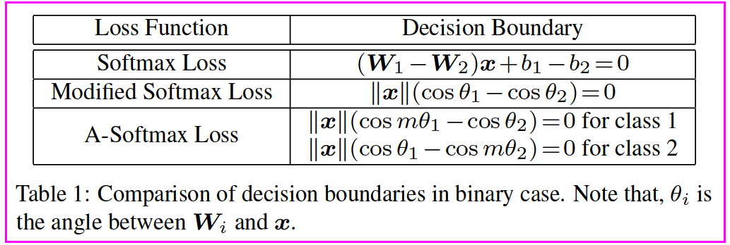
一、Softmax Loss

$$L_i=-\log \frac{e^{W_{y_i}^T{x}_i+b_{y_i}}}{{\sum }_j{e}^{W_j^T{x}_i+b_j}}=-\log \frac{e^{\Vert W_{y_i}\Vert \Vert x_i\Vert \cos ({\theta }_{y_i},i)+b_{y_i}}}{{\sum }_j{e}^{\Vert W_j\Vert \Vert x_i\Vert \cos ({\theta }_j,i)+b_j}}$$

二、SphereFace Loss

将 $W$ 归一化到 $1$，且不考虑偏置项，即 $b_j=0$，则上式变成：
$$L_{\text{modified}}=\frac{1}{N}\sum _i-\log (\frac{e^{\Vert x_i\Vert \cos ({\theta }_{y_i},i)}}{{\sum }_j{e}^{\Vert x_i\Vert \cos ({\theta }_j,i)}})$$

其中 $\theta$ 为 $W$ 和 $x$ 的夹角。

为了进一步限制夹角的范围，使用 $m\theta$（其中 $\theta$ 范围为 $[0,\frac{\pi }{m}]$），上式变成

$$L_{\text{ang}}=\frac{1}{N}\sum _i-\log (\frac{e^{\Vert x_i\Vert \cos (m{\theta }_{y_i},i)}}{e^{\Vert x_i\Vert \cos (m{\theta }_{y_i},i)}+{\sum }_{j\ne y_i}{e}^{\Vert x_i\Vert \cos ({\theta }_j,i)}})$$

为了使得上式单调，引入 $\psi ({\theta }_{y_i,i})$：

$$L_{\text{ang}}=\frac{1}{N}\sum _i-\log (\frac{e^{\Vert x_i\Vert \psi ({\theta }_{y_i,i})}}{e^{\Vert x_i\Vert \psi ({\theta }_{y_i,i})}+{\sum }_{j\ne y_i}{e}^{\Vert x_i\Vert \cos ({\theta }_j,i)}})$$

其中：$\psi ({\theta }_{y_i,i})={(-1)}^k\cos (m{\theta }_{y_i,i})-2k$

代码中引入了超参数 $\lambda$，为：

$$\lambda =\max ({\lambda }_{\min },\frac{{\lambda }_{\max }}{1+0.1\times iterator})$$

其中，${\lambda }_{\min }=5$，${\lambda }_{\max }=1500$为程序中预先设定的值。

实际的 $\psi (\theta )$ 为
$$\psi ({\theta }_{y_i})=\frac{{(-1)}^k\cos (m{\theta }_{y_i})-2k+\lambda \cos ({\theta }_{y_i})}{1+\lambda }$$

对应下面代码为：

output = cos_theta * 1.0
output[index] -= cos_theta[index]*(1.0+0)/(1+self.lamb)
output[index] += phi_theta[index]*(1.0+0)/(1+self.lamb)
1
2
3

对于 $y_i$ 处的计算，
$$output(y_i)=\cos ({\theta }_{y_i})-\frac{\cos ({\theta }_{y_i})}{1+\lambda }+\frac{\psi ({\theta }_{y_i})}{1+\lambda }=\frac{\psi ({\theta }_{y_i})+\lambda \cos ({\theta }_{y_i})}{1+\lambda }=\frac{{(-1)}^k\cos (m{\theta }_{y_i})-2k+\lambda \cos ({\theta }_{y_i})}{1+\lambda }$$
和上面的公式对应。

代码

class AngleLinear(nn.Module):
    def __init__(self, in_features, out_features, m = 4, phiflag=True):
        super(AngleLinear, self).__init__()
        self.in_features = in_features
        self.out_features = out_features
        self.weight = Parameter(torch.Tensor(in_features,out_features))
        self.weight.data.uniform_(-1, 1).renorm_(2,1,1e-5).mul_(1e5)
        self.phiflag = phiflag
        self.m = m
        self.mlambda = [
            lambda x: x**0,  # cos(0*theta)=1
            lambda x: x**1,  # cos(1*theta)=cos(theta)
            lambda x: 2*x**2-1, # cos(2*theta)=2*cos(theta)**2-1
            lambda x: 4*x**3-3*x,
            lambda x: 8*x**4-8*x**2+1,
            lambda x: 16*x**5-20*x**3+5*x
        ]

    def forward(self, input):  # input为输入的特征，(B, C)，B为batchsize，C为图像的类别总数
        x = input   # size=(B,F)，F为特征长度，如512
        w = self.weight # size=(F,C)

        ww = w.renorm(2,1,1e-5).mul(1e5) #对w进行归一化，renorm使用L2范数对第1维度进行归一化，将大于1e-5的截断，乘以1e5，使得最终归一化到1.如果1e-5设置的过大，裁剪时某些很小的值最终可能小于1。注意，第0维度只对每一行进行归一化（每行平方和为1），第1维度指对每一列进行归一化。由于w的每一列为x的权重，因而此处需要对每一列进行归一化。如果要对x归一化，需要对每一行进行归一化，此时第二个参数应为0
        xlen = x.pow(2).sum(1).pow(0.5) # 对输入x求平方，而后对不同列求和，再开方，得到每行的模，最终大小为第0维的，即B(由于对x不归一化，但是计算余弦时需要归一化，因而可以先计算模。但是对于w，不太懂为何不直接使用这种方式，而是使用renorm函数？)
        wlen = ww.pow(2).sum(0).pow(0.5) # 对权重w求平方，而后对不同行求和，再开方，得到每列的模（理论上之前已经归一化，此处应该是1，但第一次运行到此处时，并不是1，不太懂），最终大小为第1维的，即C

        cos_theta = x.mm(ww) # 矩阵相乘(B,F)*(F,C)=(B,C)，得到cos值，由于此处只是乘加，故未归一化
        cos_theta = cos_theta / xlen.view(-1,1) / wlen.view(1,-1) # 对每个cos值均除以B和C，得到归一化后的cos值
        cos_theta = cos_theta.clamp(-1,1) #将cos值截断到[-1,1]之间，理论上不截断应该也没有问题，毕竟w和x都归一化后，cos值不可能超出该范围

        if self.phiflag:
            cos_m_theta = self.mlambda[self.m](cos_theta) # 通过cos_theta计算cos_m_theta，mlambda为cos_m_theta展开的结果
            theta = Variable(cos_theta.data.acos()) # 通过反余弦，计算角度theta，(B,C)
            k = (self.m*theta/3.14159265).floor() # 通过公式，计算k，(B,C)。此处为了保证theta大于k*pi/m，转换过来就是m*theta/pi，再向上取整
            n_one = k*0.0 - 1 # 通过k的大小，得到同样大小的-1矩阵，(B,C)
            phi_theta = (n_one**k) * cos_m_theta - 2*k # 通过论文中公式，得到phi_theta。(B,C)
        else:
            theta = cos_theta.acos() # 得到角度theta，(B, C)，每一行为当前特征和w的每一列的夹角
            phi_theta = myphi(theta,self.m) #
            phi_theta = phi_theta.clamp(-1*self.m,1)

        cos_theta = cos_theta * xlen.view(-1,1)  # 由于实际上不对x进行归一化，此处cos_theta需要乘以B。(B,C)
        phi_theta = phi_theta * xlen.view(-1,1)  # 由于实际上不对x进行归一化，此处phi_theta需要乘以B。(B,C)
        output = (cos_theta,phi_theta)
        return output # size=(B,C,2)


class AngleLoss(nn.Module):
    def __init__(self, gamma=0):
        super(AngleLoss, self).__init__()
        self.gamma   = gamma
        self.it = 0
        self.LambdaMin = 5.0
        self.LambdaMax = 1500.0
        self.lamb = 1500.0

    def forward(self, input, target):
        self.it += 1
        cos_theta,phi_theta = input # cos_theta，(B,C)。 phi_theta，(B,C)
        target = target.view(-1,1) #size=(B,1)

        index = cos_theta.data * 0.0 #得到和cos_theta相同大小的全0矩阵。(B,C)
        index.scatter_(1,target.data.view(-1,1),1) # 得到一个one-hot矩阵，第i行只有target[i]的值为1，其他均为0
        index = index.byte() # index为float的，转换成byte类型
        index = Variable(index)

        self.lamb = max(self.LambdaMin,self.LambdaMax/(1+0.1*self.it))  # 得到lamb
        output = cos_theta * 1.0 #size=(B,C)  # 如果直接使用output=cos_theta，可能不收敛(未测试，但其他程序中碰到过直接对输入使用[index]无法收敛，加上*1.0可以收敛的情况)
        output[index] -= cos_theta[index]*(1.0+0)/(1+self.lamb) # 此行及下一行将target[i]的值通过公式得到最终输出
        output[index] += phi_theta[index]*(1.0+0)/(1+self.lamb)

        logpt = F.log_softmax(output) # 得到概率
        logpt = logpt.gather(1,target) # 下面为交叉熵的计算（和focal loss的计算有点类似，当gamma为0时，为交叉熵）。
        logpt = logpt.view(-1)
        pt = Variable(logpt.data.exp())

        loss = -1 * (1-pt)**self.gamma * logpt
        loss = loss.mean()

        # target = target.view(-1)  # 若要简化，理论上可直接使用这两行计算交叉熵(此处未测试，在其他程序中使用后可以正常训练)
        # loss = F.cross_entropy(cos_theta, target)

        return loss
1
2
3
4
5
6
7
8
9
10
11
12
13
14
15
16
17
18
19
20
21
22
23
24
25
26
27
28
29
30
31
32
33
34
35
36
37
38
39
40
41
42
43
44
45
46
47
48
49
50
51
52
53
54
55
56
57
58
59
60
61
62
63
64
65
66
67
68
69
70
71
72
73
74
75
76
77
78
79
80
81
82
83

---

---

---

参考资料：
（原）SphereFace及其pytorch代码
SphereFace算法详解
人脸识别之SphereFace
人脸识别论文再回顾之三：sphereface
SphereFace的翻译，解读以及训练