之前已经完成了四篇关于时间序列的博客，还没有阅读过的读者请先阅读：

1. 时间序列的数据分析(一):主要成分

2. 时间序列的数据分析(二):数据趋势的计算

3. 时间序列的数据分析(三):经典时间序列分解 
4.  时间序列的数据分析(四):STL分解

今天我们来介绍一些简单有效的预测方法,这些方法虽然比较简单但有时候却非常有效，这些简单有效的预测方法通常称为朴素预测法(Naive)。

七. 朴素预测法(Naive Forecaster)

 这里我们会使用python的sktime包来实现所有的朴素预测法，Sktime 是一个基于python时间序列建模、预测工具箱,它支持时间序列预测、时间序列分类、时间序列回归和时间序列聚类等众多实用功能，sktime内置了很多常用的时间序列预测算法比如Naive Forecaster、ARIMA、Exponential Smoothing、ETS等，今天我们会使用sktime的Naive Forecaster来实现一些简单且有效的预测功能。

7.1 均值法

此方法中，所有未来值的预测值等于历史数据的平均值。我们把历史数据记作,那么所有的预测值可以表示为：

 代表基于 对的估计值, 这里的预测值都被预测为历史数据的平均值。

接下来我们要用均值法来对之前的航空公司乘客数据集进行预测，这里创建sktime的NaiveForecaster对象，同时设置“strategy”参数为“mean”,表示使用均值法来预测，predict方法的fh参数表示预测周期,这里我们要预测未来24个月的乘客数量,所以我们设置fh=np.arange(1,25)

from sktime.datasets import load_airline
from sktime.forecasting.naive import NaiveForecaster
 
#加载数据
y = load_airline()
#创建模型
forecaster = NaiveForecaster(strategy="mean")
#训练模型
forecaster.fit(y)
#预测未来
y_pred = forecaster.predict(fh=np.arange(1,25))
 
y.index = y.index.to_timestamp()
plt.figure(figsize=(10,6))
plt.plot(y.index,y.values,label='y');
plt.plot(y_pred.index,y_pred.values,label='y_pred')
plt.ylabel('Number of airline passengers')
plt.xlabel('year month')
plt.legend(loc="upper right")
plt.show();

 这里我们预测未来24个月的乘客数量都是280.298，它是我们所有历史数据的平均值,上图中蓝色的线条就是预测值。

7.2 最后值预测法

此方法中，所有未来值的预测值等于历史数据的最后一个值即：

这种方法在很多经济和金融时间序列预测中表现得非常好。这里创建sktime的NaiveForecaster对象，同时设置“strategy”参数为“last”,表示使用最后值预测法来预测。

#加载数据
y = load_airline()
#创建模型
forecaster = NaiveForecaster(strategy="last")
#训练模型
forecaster.fit(y)
#预测未来
y_pred = forecaster.predict(fh=np.arange(1,25))
 
y.index = y.index.to_timestamp()
plt.figure(figsize=(10,6))
plt.plot(y.index,y.values,label='y');
plt.plot(y_pred.index,y_pred.values,label='y_pred')
plt.ylabel('Number of airline passengers')
plt.xlabel('year month')
plt.legend(loc="upper right")
plt.show();

 这里我们预测未来24个月的乘客数量都是432，它是我们所有历史数据中的最后一个值。

7.3 季节性最后值预测法

季节性最后值预测法与最后值预测法类似，它适用于季节性变化剧烈的数据。我们将每个预测值设为同一季节的前一期观测值（例如：去年的同一个月）。那么T+h时刻的预测值可以记作：

等式中：

• m为季节性周期长度 ，
• k是 (h−1)/m 的整数部分（也就是在 T+h 时刻前预测期所包含的整年数）。

这个等式并没有看起来那么复杂，例如，对于月度数据，未来所有二月的预测值都等于前一年二月的观测值。对于季度数据，未来所有第二季度的预测值都等于前一年第二季度的观测值。相似的规则适用于其他的月份、季度和其他周期长度。

这里创建sktime的NaiveForecaster对象，同时设置:

• strategy=last 表示使用最后值预测法
• sp=12 表示季节性周期

from sktime.datasets import load_airline
from sktime.forecasting.naive import NaiveForecaster
 
#加载数据
y = load_airline()
#创建模型
forecaster = NaiveForecaster(strategy="last",sp=12)
#训练模型
forecaster.fit(y)
#预测未来
y_pred = forecaster.predict(fh=np.arange(1,25))
 
y.index = y.index.to_timestamp()
plt.figure(figsize=(10,6))
plt.plot(y.index,y.values,label='y');
plt.plot(y_pred.index,y_pred.values,label='y_pred')
plt.ylabel('Number of airline passengers')
plt.xlabel('year month')
plt.legend(loc="upper left")
plt.show();

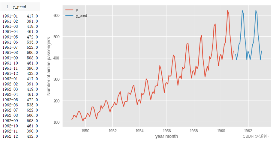
 这里我们看到我们预测的未来24个月的预测值为历史数据最后一年的历史值被重复两次的结果。

7.4 漂移法

 漂移法通过一种简单的方法来获取数据线性趋势，然后将线性趋势延长到未来的时间点，所以预测值为线性趋势的延长值，这里我们假定单位时间改变量（称作 “漂移”）等于历史数据的平均改变量，因此 T+h时刻的预测值可以表示为:

具体实现方式为将第一个观测点和最后一个观测点连成一条直线并延伸到未来预测点。这里创建sktime的NaiveForecaster对象，同时设置“strategy”参数为“drift”,表示使用漂移法来预测。

from sktime.datasets import load_airline
from sktime.forecasting.naive import NaiveForecaster
 
#加载数据
y = load_airline()
#创建模型
forecaster = NaiveForecaster(strategy="drift")
#训练模型
forecaster.fit(y)
#预测未来
y_pred = forecaster.predict(fh=np.arange(1,25))
 
y.index = y.index.to_timestamp()
plt.figure(figsize=(10,6))
plt.plot(y.index,y.values,label='y');
plt.plot(y_pred.index,y_pred.values,label='y_pred')
plt.ylabel('Number of airline passengers')
plt.xlabel('year month')
plt.legend(loc="upper left")
plt.show();

7.5 例子

下面我们用以上四种朴素预测法来预测一下google的股票价格，首先使用yfinance 包来获取股票数据,然后我们分别使用四种朴素预测法来预测2个月的google的股票价格：

import yfinance as yf
from sktime.forecasting.naive import NaiveForecaster
 
#加载数据
ticker = yf.Ticker('goog')
data = ticker.history(start='2020-05-1',end='2021-06-1')
data=data[['Close']]
data.index = data.index.to_period("D")
 
# 均值法
y_pred_mean =NaiveForecaster(strategy="mean").fit_predict(data,fh=np.arange(1,61))
 
# 最后值法
y_pred_last =NaiveForecaster(strategy="last").fit_predict(data,fh=np.arange(1,61))
 
# 季节性最后值法
y_pred_seasonal =NaiveForecaster(strategy="last",sp=1).fit_predict(data,fh=np.arange(1,61))
 
# 漂移法
y_pred_drift =NaiveForecaster(strategy="drift").fit_predict(data,fh=np.arange(1,61))
 
data.index = data.index.to_timestamp()
y_pred_mean.index = y_pred_mean.index.to_timestamp()
y_pred_last.index = y_pred_last.index.to_timestamp()
y_pred_seasonal.index = y_pred_seasonal.index.to_timestamp()
y_pred_drift.index = y_pred_drift.index.to_timestamp()
plt.figure(figsize=(12,6))
plt.plot(data.index,data.Close,label='y');
plt.plot(y_pred_mean.index,y_pred_mean.values,label='y_pred_mean')
plt.plot(y_pred_last.index,y_pred_last.values,label='y_pred_last')
plt.plot(y_pred_seasonal.index,y_pred_seasonal.values,label='y_pred_seasonal')
plt.plot(y_pred_drift.index,y_pred_drift.values,label='y_pred_drift')
plt.title('Google Stock Price (2020-05-1 to 2021-06-1) ')
plt.ylabel('Stock Price($)')
plt.xlabel('date')
plt.legend(loc="upper left")
plt.show();

这里需要说明的是股票数据属于一种随机游走的随机过程，它不存在季节性周期项，股票的价格由受诸多外在因素的影响如宏观经济环境，企业自身的经营业绩等，所以股票价格更难以预测，因此不能套用大多基于季节性的预测算法如ARIMA等。然而简单的朴素预测算法如drift,有时候会却有较好的预测效果，有兴趣的读者可以尝试一下。

总结

今天我们解释了4种最简单的朴素预测法：均值法，最后值法，季节性最后值法，漂移法，朴素预测法虽然很简单但有时候也会有较好的预测效果，如季节性周期变化很明显的时候我们可以使用季节性最后值法，当遇到类似随机游走型的时间序列如股票数据时使用漂移法有时候也会有较好的预测效果。有兴趣的读者可以自己尝试一下使用yfinance 包来下载美国的股票数据如：特斯拉，苹果，谷歌的股票代码:tsla、aapl、goog来进行研究。

参考资料

NaiveForecaster — sktime documentation